作者:樵溪子,清华大学,清华大学深圳国际研究生院,清华-伯克利深圳学院,硕士在读
审校:刘兴禄,清华大学,清华大学深圳国际研究生院,清华-伯克利深圳学院,硕士在读
设施选址问题是经典的运筹优化问题,常见模型有:
- 覆盖问题(Covering Model)
- 最大覆盖问题(Maximum Covering Model)
- p p p-中心问题(p-cernter Problem)
- p p p-扩散问题(p-dispersion Problem)
- p p p-中位问题(p-median Problem)
本文对以上5个模型进行了梳理,并给出了相应的算例、完整实现代码以及结果的可视化。本文可以为初学者提供较好的学习参考。
本文的模型参考自文献:
Ho-Yin Mak and Zuo-Jun Max Shen (2016), “Integrated Modeling for Location Analysis”, Foundations and Trends in Technology, Information and Operations Management: Vol. 9, No. 1-2, pp 1–152. DOI: 10.1561/0200000037
一、覆盖问题(Covering Model)
1、问题描述
假设有一个需求点的位置集合和一个设施的位置集合,且已知每个设施的服务范围。在
满足覆盖所有需求点顾客的前提下,选取若干个点建造设施,以使得建设总成本最小。
2、模型构建
(1) 参数
- I I I:需求点位置集合;
- J J J:潜在设施位置集合;
- f j f_{j} fj:在 j j j点建造设施的成本。
-
a
i
j
a_{ij}
aij:表示覆盖范围,其具体含义如下:
a i , j = { 1 , 在 j 点建造设施能够覆盖需求点 i 0 , 其他 a_{i,j}= \begin{cases} 1, & 在j点建造设施能够覆盖需求点i \\ 0 , & 其他 \end{cases} ai,j={1,0,在j点建造设施能够覆盖需求点i其他
(2) 决策变量
X j = { 1 , 在 j 点建造设施 0 , 其他 X_{j}= \begin{cases} 1, & 在j点建造设施\\ 0, & 其他 \end{cases} Xj={1,0,在j点建造设施其他
(3)整数规划模型
min ∑ j ∈ J f j X j s . t . ∑ j ∈ J a i , j X j ⩾ 1 ∀ i ∈ I , X j ∈ { 0 , 1 } , ∀ j ∈ J . \begin{aligned} \min \quad &\sum_{j \in J} f_{j} X_{j} && \\ s.t. \quad &\sum_{j\in J}a_{i,j}X_{j} \geqslant 1 \quad &&\forall i \in I, \\ &X_{j} \in \{0,1\}, \quad &&\forall j \in J. \end{aligned} mins.t.j∈J∑fjXjj∈J∑ai,jXj⩾1Xj∈{0,1},∀i∈I,∀j∈J.
3、代码实现
from gurobipy import *
import random
import numpy as np

# Parameters
num_points = 5 							# I: set of the demand points
num_facilities = 10  					# J: set of possible facility location
setup_cost = [3,2,3,1,3,3,4,3,2,4]  	# f: cost of locate each facility
np.random.seed(0)
cover = np.random.randint(2,size=(num_points,num_facilities)) # a:facility at j can cover point i

# Create a new model
m = Model("Covering Model")

# Create variables
select = m.addVars(num_facilities, vtype=GRB.BINARY, name='Select') # X

# Add constraints
m.addConstrs((quicksum((cover[i,j] * select[j]) for j in range(num_facilities)) >= 1 for i in range(num_points)), name='Cover')

# Set objective
m.setObjective(select.prod(setup_cost), GRB.MINIMIZE)

m.optimize()

for v in m.getVars():
    if v.x > 0 :
        print('%s %g' % (v.varName, v.x))

print('obj:%g' % m.objVal)
4、运行结果
Gurobi Optimizer version 9.5.2 build v9.5.2rc0 (mac64[arm])
Thread count: 8 physical cores, 8 logical processors, using up to 8 threads
Optimize a model with 5 rows, 10 columns and 30 nonzeros
Model fingerprint: 0x0f7f480f
Variable types: 0 continuous, 10 integer (10 binary)
Coefficient statistics:
  Matrix range     [1e+00, 1e+00]
  Objective range  [1e+00, 4e+00]
  Bounds range     [1e+00, 1e+00]
  RHS range        [1e+00, 1e+00]
Found heuristic solution: objective 6.0000000
Presolve removed 5 rows and 10 columns
Presolve time: 0.00s
Presolve: All rows and columns removed

Explored 0 nodes (0 simplex iterations) in 0.00 seconds (0.00 work units)
Thread count was 1 (of 8 available processors)

Solution count 2: 3 6

Optimal solution found (tolerance 1.00e-04)
Best objective 3.000000000000e+00, best bound 3.000000000000e+00, gap 0.0000%
Select[3] 1
Select[8] 1
obj:3
二、最大覆盖问题(Maximum Covering Model)
1、问题描述
假设有一个需求点的位置集合,且已知每个设施的服务范围、每个需求点的客户人数以及设施总数。
在设施总数一定的前提下,选取建造设施的位置以及提供服务的站点,以使得被服务到的客户人数最大。
2、模型构建
(1) 参数
I
I
I:需求点位置集合
P
P
P:设施总数
h
i
h_{i}
hi:在i点的客户人数
a
i
j
=
{
1
,
在
j
点建造设施能够覆盖需求点
i
0
,
其他
a_{ij}= \begin{cases} 1, & 在j点建造设施能够覆盖需求点i \\ 0 , & 其他 \end{cases}
aij={1,0,在j点建造设施能够覆盖需求点i其他
(2) 决策变量
X
i
=
{
1
,
在
i
点建造设施
0
,
其他
Z
i
=
{
1
,
为
i
点提供服务
0
,
其他
X_{i}= \begin{cases} 1, & 在i点建造设施\\ 0, & 其他 \end{cases} \\ Z_{i}= \begin{cases} 1, & 为i点提供服务\\ 0, & 其他 \end{cases}
Xi={1,0,在i点建造设施其他Zi={1,0,为i点提供服务其他
(3)整数规划模型
max
∑
i
∈
I
h
i
Z
i
s
.
t
.
∑
i
∈
I
X
i
=
P
,
∑
j
∈
I
a
i
j
X
j
≥
Z
i
,
∀
i
∈
I
,
X
i
,
Z
i
∈
{
0
,
1
}
,
∀
i
∈
I
.
\begin{aligned} \text{max} & \sum_{i \in I} h_{i} Z_{i} &&\\ s.t. \quad &\sum_{i\in I}X_{i} = P, &&\\ &\sum_{j\in I}a_{ij}X_{j} \geq Z_{i}, \quad&&\forall i \in I, \\ &X_{i} ,Z_{i}\in \{0,1\}, \quad &&\forall i \in I. \end{aligned}
maxs.t.i∈I∑hiZii∈I∑Xi=P,j∈I∑aijXj≥Zi,Xi,Zi∈{0,1},∀i∈I,∀i∈I.
3、代码实现
from gurobipy import *
import random
import numpy as np

# Parameters
# Facility is the scarce resources, so num_points is bigger than num_located
# Set of possible facility location is the set of the demand points ( J == I )
num_points = 10 # I: set of the demand points
num_located = 5 # P: number of facility

np.random.seed(0)
num_people = np.random.randint(6,size = num_points)  # h
cover = np.random.randint(2,size=(num_points,num_points)) # a

# Create a new model
m = Model("Maximum Covering Model")

# Create variables
select = m.addVars(num_points, vtype=GRB.BINARY, name='Select') # X
serve = m.addVars(num_points, vtype=GRB.BINARY, name='Serve') # Z

# Add constraints
m.addConstrs((quicksum((cover[(i,j)] * select[j]) for j in range(num_points)) >= serve[i] for i in range(num_points)), name='Cover_before_serve')
m.addConstr((quicksum(select) == num_located), name='Num_limit')  # addConstrs --> error: Missing Constraint Index


# Set objective
m.setObjective(quicksum(serve[i]*num_people[i] for i in range(num_points)), GRB.MAXIMIZE)

m.write("lp--Max_Covering_Problem.lp")
m.optimize()

# Print results
selected = []
served = []
for i in select.keys():
    if select[i].x > 0:
        selected.append(i)
    if serve[i].x > 0:
        served.append(i)

print("Selected position = ", selected)
print("Served position = ", served)
print('Max served number = %g' % m.objVal)
4、运行结果
Gurobi Optimizer version 9.5.2 build v9.5.2rc0 (mac64[arm])
Thread count: 8 physical cores, 8 logical processors, using up to 8 threads
Optimize a model with 11 rows, 20 columns and 72 nonzeros
Model fingerprint: 0xbd3d5b75
Variable types: 0 continuous, 20 integer (20 binary)
Coefficient statistics:
  Matrix range     [1e+00, 1e+00]
  Objective range  [1e+00, 5e+00]
  Bounds range     [1e+00, 1e+00]
  RHS range        [5e+00, 5e+00]
Found heuristic solution: objective 29.0000000

Explored 0 nodes (0 simplex iterations) in 0.00 seconds (0.00 work units)
Thread count was 1 (of 8 available processors)

Solution count 1: 29

Optimal solution found (tolerance 1.00e-04)
Best objective 2.900000000000e+01, best bound 2.900000000000e+01, gap 0.0000%
Selected position =  [2, 3, 4, 5, 9]
Served position =  [0, 1, 3, 4, 5, 6, 7, 8, 9]
Max served number = 29
三、 p p p-中心问题( p p p-cernter Problem)
1、问题描述
假设有一个需求点的位置集合,且已知设施总数。
在设施总数一定的前提下,确定在哪些需求点建造设施,以及需求点与设施的对应分配关系,使得所有需求点到达其所属设施的距离最大值最小。
2、模型构建
(1) 参数
I
I
I:需求点位置集合
P
P
P:设施总数
d
i
j
d_{ij}
dij:
i
i
i点与
j
j
j点之间的距离
(2) 决策变量
X
i
=
{
1
,
在
i
点建造设施
0
,
其他
X_{i}= \begin{cases} 1, & 在i点建造设施\\ 0, & 其他 \end{cases}
Xi={1,0,在i点建造设施其他
Y
i
j
=
{
1
,
将
i
点分配给
j
点
0
,
其他
Y_{ij}= \begin{cases} 1, & 将i点分配给j点\\ 0, & 其他 \end{cases}
Yij={1,0,将i点分配给j点其他
- w w w: 所有需求点到达其所属设施的距离最大值。
(3)建模
min
w
s
.
t
.
∑
i
∈
I
X
i
=
P
,
Y
i
j
≤
X
j
,
∀
i
,
j
∈
I
,
∑
j
∈
I
Y
i
j
=
1
,
∀
i
∈
I
,
∑
j
∈
I
d
i
j
Y
i
j
≤
w
,
∀
i
,
j
∈
I
,
X
i
,
Y
i
j
∈
{
0
,
1
}
,
∀
i
,
j
∈
I
.
\begin{aligned} \text{min} &\quad w &&\\ s.t. \quad &\sum_{i\in I}X_{i} = P, &&\\ &Y_{ij} \leq X_{j}, \quad&&\forall i,j \in I, \\ &\sum_{j\in I}Y_{ij} = 1, \quad &&\forall i \in I, \\ &\sum_{j\in I}d_{ij}Y_{ij} \leq w, \quad &&\forall i,j \in I, \\ &X_{i} ,Y_{ij}\in \{0,1\}, \quad &&\forall i,j \in I. \end{aligned}
mins.t.wi∈I∑Xi=P,Yij≤Xj,j∈I∑Yij=1,j∈I∑dijYij≤w,Xi,Yij∈{0,1},∀i,j∈I,∀i∈I,∀i,j∈I,∀i,j∈I.
3、代码实现
from itertools import product
from gurobipy import *
import numpy as np
from math import sqrt
import random
import matplotlib.pyplot as plt

# Parameters
num_points = 10
random.seed(0)
points = [(random.random(), random.random()) for i in range(num_points)]
num_located = 2  # P: number of located facility in the end
cartesian_prod = list(product(range(num_points), range(num_points)))

# Compute distance
def compute_distance(loc1, loc2):
    dx = loc1[0] - loc2[0]
    dy = loc1[1] - loc2[1]
    return sqrt(dx*dx + dy*dy)
dist = {(i,j): compute_distance(points[i], points[j]) for i, j in cartesian_prod}

# Create a new model
m = Model("p-center Problem")

# Create variables
select = m.addVars(num_points, vtype=GRB.BINARY, name='Select') # X
assign = m.addVars(cartesian_prod, vtype=GRB.BINARY, name='Assign') # Y
omega= m.addVar(lb=0, ub=GRB.INFINITY, vtype=GRB.CONTINUOUS, name='Omega') #

# Add constraints
m.addConstr((quicksum(select) == num_located), name='Num_limit')
m.addConstrs((assign[(i,j)] <= select[j] for i,j in cartesian_prod), name='Assign_before_locate')
m.addConstrs((quicksum(assign[(i,j)] for j in range(num_points)) == 1 for i in range(num_points)), name='Unique_assign')
m.addConstr((assign.prod(dist) <= omega), name='Min_distance')

# Set objective
m.setObjective(omega, GRB.MINIMIZE)

m.write("lp--p_center_Problem.lp")
m.optimize()

# Print results
selected = []
assigned = []
for i in select.keys():
    if select[i].x > 0:
        selected.append(i)
for i in assign.keys():
    if assign[i].x > 0:
        assigned.append(i)
print("Selected positions = ", selected)
print("Assigned relationships = ", assigned)
print('Min distance = %g' % m.objVal)

# Plot
node_facility = []
node_ponit = []
for key in select.keys():
    if select[key].x > 0:
        node_facility.append(points[key])
    else:
        node_ponit.append(points[key])

plt.figure(figsize=(4,4))
plt.title('p-center Problem(P=2,I=10)')
plt.scatter(*zip(*node_facility), c='Red', marker=',',s=20,label = 'Facility')
plt.scatter(*zip(*node_ponit), c='Orange', marker='o',s=15, label = 'Ponit')
assignments = [p for p in assign.keys() if assign[p].x > 0.5]
for p in assignments:
    pts = [points[p[0]], points[p[1]]]
    plt.plot(*zip(*pts), c='Black', linewidth=0.5)

plt.grid(False)
plt.legend(loc='best', fontsize = 10)
plt.show()
4、运行结果
Gurobi Optimizer version 9.5.2 build v9.5.2rc0 (mac64[arm])
Thread count: 8 physical cores, 8 logical processors, using up to 8 threads
Optimize a model with 112 rows, 111 columns and 401 nonzeros
Model fingerprint: 0x1696fd10
Variable types: 1 continuous, 110 integer (110 binary)
Coefficient statistics:
  Matrix range     [1e-01, 1e+00]
  Objective range  [1e+00, 1e+00]
  Bounds range     [1e+00, 1e+00]
  RHS range        [1e+00, 2e+00]
Found heuristic solution: objective 4.4338834
Presolve removed 1 rows and 1 columns
Presolve time: 0.00s
Presolved: 111 rows, 110 columns, 310 nonzeros
Found heuristic solution: objective 2.3073713
Variable types: 0 continuous, 110 integer (110 binary)

Root relaxation: objective 1.895186e+00, 53 iterations, 0.00 seconds (0.00 work units)

    Nodes    |    Current Node    |     Objective Bounds      |     Work
 Expl Unexpl |  Obj  Depth IntInf | Incumbent    BestBd   Gap | It/Node Time

*    0     0               0       1.8951858    1.89519  0.00%     -    0s

Explored 1 nodes (53 simplex iterations) in 0.01 seconds (0.00 work units)
...
Best objective 1.895185783874e+00, best bound 1.895185783874e+00, gap 0.0000%
Selected positions =  [0, 2]
Assigned relationships =  [(0, 0), (1, 2), (2, 2), (3, 2), (4, 2), (5, 0), (6, 2), (7, 2), (8, 0), (9, 0)]
Min distance = 1.89519
可视化的结果如下图:
四、 p p p-扩散问题( p p p-dispersion Problem)
1、问题描述
- 假设有一个需求点的位置集合,且已知设施总数。在设施总数一定的前提下,确定在哪些需求点建造设施,使得所有需求点之间的距离最小值最大。
- 应用场景:发射井之间的距离越远,攻击者在一次打击中摧毁多个发射井的几率就越小。如果快餐加盟店分散在整个城市,总销售额可能会更高。
2、模型构建
(1) 参数
I
I
I:需求点位置集合
P
P
P:设施总数
d
i
j
d_{ij}
dij:i点与j点之间的距离
(2) 决策变量
D
m
i
n
D_{min}
Dmin:一对节点之间的最短距离
X
i
=
{
1
,
在
i
点建造设施
0
,
其他
X_{i}= \begin{cases} 1, & 在i点建造设施\\ 0, & 其他 \end{cases} \\
Xi={1,0,在i点建造设施其他
(3)建模
max
D
m
i
n
(
1
)
s
.
t
.
∑
i
∈
I
X
i
=
P
,
(
2
)
X
j
X
k
d
j
k
≥
D
m
i
n
X
j
X
k
,
∀
j
,
k
∈
I
,
(
3
)
X
i
∈
{
0
,
1
}
,
∀
i
∈
I
.
(
4
)
\begin{aligned} \text{max} & \quad D_{min} &&&& (1)\\ s.t. \quad &\sum_{i\in I}X_{i} = P, && && (2)\\ &X_{j}X_{k}d_{jk} \geq D_{min}X_{j}X_{k}, \quad &&\forall j,k \in I, && (3)\\ &X_{i} \in \{0,1\}, \quad &&\forall i \in I. && (4) \end{aligned}
maxs.t.Dmini∈I∑Xi=P,XjXkdjk≥DminXjXk,Xi∈{0,1},∀j,k∈I,∀i∈I.(1)(2)(3)(4)
注意到,上面模型中的约束(3)含有非线性项
X
j
X
k
X_{j}X_{k}
XjXk。该非线性项为两个0-1变量相乘。我们可以通过引入逻辑约束将其等价线性化,线性化后的约束如下:
(
2
−
X
j
−
X
k
)
M
+
d
j
k
≥
D
m
i
n
,
∀
j
,
k
∈
I
.
\begin{aligned} (2-X_{j}-X_{k})M + d_{jk} \geq D_{min}, \forall j,k \in I. \end{aligned}
(2−Xj−Xk)M+djk≥Dmin,∀j,k∈I.
当然,也可以使用之前的推文中介绍的方法进行等价线性化。推文链接如下:
【】
但是注意,本文提供的线性化方法,不需要引入额外的辅助变量,因此,推荐使用本文的方法。
3、代码实现
from itertools import product
from gurobipy import *
import numpy as np
from math import sqrt
import random
import matplotlib.pyplot as plt

# Parameters
num_points = 10
random.seed(0)
points = [(random.random(), random.random()) for i in range(num_points)]
num_located = 2  # P: number of located facility in the end
cartesian_prod = list(product(range(num_points), range(num_points)))
M = 100

# Compute distance
def compute_distance(loc1, loc2):
    dx = loc1[0] - loc2[0]
    dy = loc1[1] - loc2[1]
    return sqrt(dx*dx + dy*dy)
dist = {(i,j): compute_distance(points[i], points[j])
    for i, j in cartesian_prod
    if i != j }

# Create a new model
m = Model("p-dispersion Problem")

# Create variables
select = m.addVars(num_points, vtype=GRB.BINARY, name='Select') # X
D_min = m.addVar(lb=0, ub=GRB.INFINITY, obj=1, vtype=GRB.CONTINUOUS, name='D_min')

# Add constraints
m.addConstr(quicksum(select) == num_located, name='Num_limit')
m.addConstrs(((2 - select[i] - select[j])* M + dist[i,j] >= D_min for i,j in cartesian_prod if i != j), name='Min_dist')
#m.addConstrs(((2 - select[i] - select[j])* M + (select[i] + select[j]) * dist[i,j] >= 2 * D_min for i,j in cartesian_prod if i != j), name='Min_dist')  # equal to the formula above

# Set objective
m.setObjective(D_min, GRB.MAXIMIZE)

m.write("lp-p_dispersion_Problem.lp")
m.optimize()

# Print results
selected = []
for i in select.keys():
    if select[i].x > 0:
        selected.append(i)
print("Selected positions = ", selected)
print('D_min = %g' % D_min.x)

# Plot
facility = []
for key in select.keys():
    if select[key].x > 0:
        facility.append(points[key])

plt.figure(figsize=(4,4))
plt.title('p-dispersion Problem(P=5,I=10)')
plt.scatter(*zip(*points), c='Pink', marker='o',s=15, label = 'Ponit')
plt.scatter(*zip(*facility), c='Red', marker=',',s=20, label = 'Facility')
plt.grid(False)
plt.legend(loc='best', fontsize = 10)
plt.show()
4、运行结果
Gurobi Optimizer version 9.5.2 build v9.5.2rc0 (mac64[arm])
Thread count: 8 physical cores, 8 logical processors, using up to 8 threads
Optimize a model with 91 rows, 11 columns and 280 nonzeros
Model fingerprint: 0xb07db2f0
Variable types: 1 continuous, 10 integer (10 binary)
Coefficient statistics:
  Matrix range     [1e+00, 1e+02]
  Objective range  [1e+00, 1e+00]
  Bounds range     [1e+00, 1e+00]
  RHS range        [5e+00, 2e+02]
Found heuristic solution: objective 0.1718957
Presolve removed 45 rows and 0 columns
Presolve time: 0.00s
Presolved: 46 rows, 11 columns, 145 nonzeros
Variable types: 1 continuous, 10 integer (10 binary)

Root relaxation: objective 1.001990e+02, 21 iterations, 0.00 seconds (0.00 work units)

    Nodes    |    Current Node    |     Objective Bounds      |     Work
 Expl Unexpl |  Obj  Depth IntInf | Incumbent    BestBd   Gap | It/Node Time

     0     0  100.19898    0   10    0.17190  100.19898      -     -    0s
H    0     0                       0.1817861  100.19898      -     -    0s
H    0     0                       0.2341288  100.19898      -     -    0s
H    0     0                       0.2601163   57.43551      -     -    0s
...
Optimal solution found (tolerance 1.00e-04)
Best objective 2.601163466179e-01, best bound 2.601163466179e-01, gap 0.0000%
Selected positions =  [0, 4, 5, 6, 7]
D_min = 0.260116
我们将求解结果进行可视化,结果如下。下图中,共有10个候选点,其中,红色的点为被选中的点。
五、 p p p-中位问题( p p p-median Problem)
1、问题描述
假设有一个需求点的位置集合,且已知每个需求点的客户人数和设施总数。
在设施总数一定的前提下,确定在哪些需求点建造设施,以及需求点与设施的对应分配关系,使得所有需求点的客户到达其所属设施的距离总和最小。
2、模型构建
(1) 参数
I
I
I:需求点位置集合;
h
i
h_{i}
hi:在i点的客户人数;
P
P
P:设施总数;
d
i
j
d_{ij}
dij:
i
i
i点与
j
j
j点之间的距离。
(2) 决策变量
X
i
=
{
1
,
在
i
点建造设施
0
,
其他
Y
i
j
=
{
1
,
将
i
点分配给
j
点
0
,
其他
X_{i}= \begin{cases} 1, & 在i点建造设施\\ 0, & 其他 \end{cases} \\ Y_{ij}= \begin{cases} 1, & 将i点分配给j点\\ 0, & 其他 \end{cases}
Xi={1,0,在i点建造设施其他Yij={1,0,将i点分配给j点其他
(3)建模
min
∑
i
,
j
∈
I
h
i
d
i
j
Y
i
j
s
.
t
.
∑
i
∈
I
X
i
=
P
,
Y
i
j
≤
X
j
,
∀
i
,
j
∈
I
,
∑
j
∈
I
Y
i
j
=
1
,
∀
i
∈
I
,
X
i
,
Y
i
j
∈
{
0
,
1
}
,
∀
i
,
j
∈
I
.
\begin{aligned} \text{min} \quad &\sum_{i,j\in I}h_{i}d_{ij}Y_{ij}&& \\ s.t. \quad &\sum_{i\in I}X_{i} = P, && \\ &Y_{ij} \leq X_{j}, \quad&& \forall i,j \in I, \\ &\sum_{j\in I}Y_{ij} = 1, \quad &&\forall i \in I, \\ &X_{i} ,Y_{ij}\in \{0,1\}, \quad &&\forall i,j \in I. \end{aligned}
mins.t.i,j∈I∑hidijYiji∈I∑Xi=P,Yij≤Xj,j∈I∑Yij=1,Xi,Yij∈{0,1},∀i,j∈I,∀i∈I,∀i,j∈I.
3、代码实现
from itertools import product
from gurobipy import *
import numpy as np
from math import sqrt
import random
import matplotlib.pyplot as plt

# Parameters
num_points = 10
random.seed(0)
points = [(random.random(), random.random()) for i in range(num_points)]
num_located = 2  # P: number of located facility in the end
cartesian_prod = list(product(range(num_points), range(num_points)))
np.random.seed(0)
num_people = np.random.randint(low=1,high=6,size = num_ponits)  # h

# Compute distance
def compute_distance(loc1, loc2):
    dx = loc1[0] - loc2[0]
    dy = loc1[1] - loc2[1]
    return sqrt(dx*dx + dy*dy)
dist = {(i,j): compute_distance(points[i], points[j]) for i, j in cartesian_prod}

# Create a new model
m = Model("p-median Problem")

# Create variables
select = m.addVars(num_points, vtype=GRB.BINARY, name='Select') # X
assign = m.addVars(cartesian_prod, vtype=GRB.BINARY, name='Assign') # Y

# Add constraints
m.addConstr((quicksum(select) == num_located), name='Num_limit')
m.addConstrs((assign[i,j] <= select[j] for i,j in cartesian_prod), name='Assign_before_locate')
m.addConstrs((quicksum(assign[i,j] for j in range(num_points)) == 1 for i in range(num_points)), name='Unique_assign')

# Set objective
m.setObjective(quicksum(num_people[i]*dist[i,j]*assign[i,j] for i,j in cartesian_prod), GRB.MINIMIZE)

#m.write("lp--p_median_Problem.lp")
m.optimize()

# Print results
selected = []
assigned = []
for i in select.keys():
    if select[i].x > 0:
        selected.append(i)
for i in assign.keys():
    if assign[i].x > 0:
        assigned.append(i)
print("Selected positions = ", selected)
print("Assigned relationships = ", assigned)
print('Objvalue = %g' % m.objVal)

# Plot
node_facility = []
node_ponit = []
for key in select.keys():
    if select[key].x > 0:
        node_facility.append(points[key])
    else:
        node_ponit.append(points[key])

plt.figure(figsize=(4,4))
plt.title('p-median Problem(P=2,I=10)')
plt.scatter(*zip(*node_facility), c='Red', marker=',',s=20,label = 'Facility')
plt.scatter(*zip(*node_ponit), c='Orange', marker='o',s=15, label = 'Ponit')
assignments = [p for p in assign.keys() if assign[p].x > 0.5]
for p in assignments:
    pts = [points[p[0]], points[p[1]]]
    plt.plot(*zip(*pts), c='Black', linewidth=0.5)

plt.grid(False)
plt.legend(loc='best', fontsize = 10)
plt.show()
4、运行结果文章来源:https://www.toymoban.com/news/detail-416355.html
Gurobi Optimizer version 9.5.2 build v9.5.2rc0 (mac64[arm])
Thread count: 8 physical cores, 8 logical processors, using up to 8 threads
Optimize a model with 111 rows, 110 columns and 310 nonzeros
Model fingerprint: 0x014c5262
Variable types: 0 continuous, 110 integer (110 binary)
Coefficient statistics:
  Matrix range     [1e+00, 1e+00]
  Objective range  [1e-01, 4e+00]
  Bounds range     [1e+00, 1e+00]
  RHS range        [1e+00, 2e+00]
Found heuristic solution: objective 14.2576250
Presolve time: 0.00s
Presolved: 111 rows, 110 columns, 310 nonzeros
Variable types: 0 continuous, 110 integer (110 binary)
Found heuristic solution: objective 7.7610282

Root relaxation: objective 6.144313e+00, 54 iterations, 0.00 seconds (0.00 work units)

    Nodes    |    Current Node    |     Objective Bounds      |     Work
 Expl Unexpl |  Obj  Depth IntInf | Incumbent    BestBd   Gap | It/Node Time

*    0     0               0       6.1443125    6.14431  0.00%     -    0s

Explored 1 nodes (54 simplex iterations) in 0.01 seconds (0.00 work units)
Thread count was 8 (of 8 available processors)
...
Selected positions =  [0, 2]
Assigned relationships =  [(0, 0), (1, 2), (2, 2), (3, 2), (4, 2), (5, 0), (6, 2), (7, 2), (8, 0), (9, 0)]
Objvalue = 6.14431
Numbers of people =  [5 1 4 4 4 2 4 3 5 1]
运行结果的可视化如下: 文章来源地址https://www.toymoban.com/news/detail-416355.html
参考文献
- Ho-Yin Mak and Zuo-Jun Max Shen (2016), “Integrated Modeling for Location Analysis”, Foundations and Trends in Technology, Information and Operations Management: Vol. 9, No. 1-2, pp 1–152. DOI: 10.1561/0200000037
到了这里,关于优化|五个经典设施选址模型的详解及其实践:Python调用Gurobi实现的文章就介绍完了。如果您还想了解更多内容,请在右上角搜索TOY模板网以前的文章或继续浏览下面的相关文章,希望大家以后多多支持TOY模板网!


![[ 注意力机制 ] 经典网络模型1——SENet 详解与复现](https://imgs.yssmx.com/Uploads/2024/01/807521-1.png)
![[ 可视化 ] 经典网络模型 —— Grad-CAM 详解与复现](https://imgs.yssmx.com/Uploads/2024/02/784097-1.png)


