传统目标检测实战:HOG+SVM
1. 前言
1.1 传统和深度
在深度学习出现之前,传统的目标检测方法大概分为区域选择(滑窗)、特征提取(SIFT、HOG等)、**分类器(SVM、Adaboost等)**三个部分,其主要问题有两方面:一方面滑窗选择策略没有针对性、时间复杂度高,窗口冗余;另一方面手工设计的特征鲁棒性较差。自深度学习出现之后,目标检测取得了巨大的突破,最瞩目的两个方向有:
- 以RCNN为代表的基于Region Proposal的深度学习目标检测算法(RCNN,SPP-NET,Fast-RCNN,Faster-RCNN等),它们是two-stage的,需要先使用启发式方法(selective search)或者CNN网络(RPN)产生Region Proposal,然后再在Region Proposal上做分类与回归。
- 以YOLO为代表的基于回归方法的深度学习目标检测算法(YOLO,SSD等),其仅仅使用一个CNN网络直接预测不同目标的类别与位置。
1.2 何为传统目标检测
首先我们先来了解一下什么是目标检测?简单来说就是把存在的目标从图片中找到并识别出来。我们发现这对于我们人来说十分简单,但对于计算机而言,它是怎么做到的呢?
- 传统目标检测方法分为三部分:区域选择 → 特征提取 → 分类器
即首先在给定的图像上选择一些候选的区域,然后对这些区域提取特征,最后使用训练的分类器进行分类。下面我们对这三个阶段分别进行介绍。
-
区域选择:这一步是为了对目标的位置进行定位。由于目标可能出现在图像的任何位置,而且目标的大小、长宽比例也不确定,所以最初采用滑动窗口的策略对整幅图像进行遍历,而且需要设置不同的尺度,不同的长宽比。这种穷举的策略虽然包含了目标所有可能出现的位置,但是缺点也是显而易见的:时间复杂度太高,产生冗余窗口太多,这也严重影响后续特征提取和分类的速度和性能。(实际上由于受到时间复杂度的问题,滑动窗口的长宽比一般都是固定的设置几个,所以对于长宽比浮动较大的多类别目标检测,即便是滑动窗口遍历也不能得到很好的区域)。
-
特征提取:由于目标的形态多样性,光照变化多样性,背景多样性等因素使得设计一个鲁棒的特征并不是那么容易。然而提取特征的好坏直接影响到分类的准确性。(这个阶段常用的特征有SIFT、HOG等)
-
分类器:主要有SVM,Adaboost等。
1.3 传统目标检测方法不足
总结一下,传统目标检测存在的两个主要问题:
- 基于滑动窗口的区域选择策略没有针对性,时间复杂度高,窗口冗余;
- 手工设计的特征对于多样性的变化并没有很好的鲁棒性。
2. 先验知识
- 机器视觉特征简单介绍:HOG、SIFT、SURF、ORB、LBP、HAAR
- skimage.feature–corner_harris、hog、local_binary_pattern说明
- SVM很好理解,就是分类器
3. 项目框架
**本文主要是针对裂缝目标检测的项目。**也可扩展到其他的目标检测。!!!
3.1 文件架构

- data代表数据文件夹,下有img(原始图像有正样本(有裂缝)和负样本(无裂缝))、feature(对原始图像提取特征后,得到正样本特征和负样本特征)、model(保存训练好的分类器)、result(预测的结果)和test_img(预测时所用到的图像)。
- 其余的py文件,下面详细介绍。
3.2 方法简要介绍


4. 工具函数(utils.py)
from skimage.feature import hog, local_binary_pattern

# settings for LBP
radius = 3
n_points = 8 * radius

# settings for HOG
ppc = (32, 32)
cpb = (3, 3)


def get_hog_feature(img):
    return hog(img, orientations=9, pixels_per_cell=ppc, cells_per_block=cpb, block_norm='L1', transform_sqrt=False, feature_vector=True)

def get_lbp_feature(img):
    return local_binary_pattern(img, n_points, radius)


def sliding_window(image, window_size, step_size):
    for row in range(0, image.shape[0], step_size[0]):
        for col in range(0, image.shape[1], step_size[1]):
            yield (row, col, image[row:row + window_size[0], col:col + window_size[1]])


def overlapping_area(detection_1, detection_2, show = False):
    '''
    计算两个检测区域覆盖大小,detection:(x, y, pred_prob, width, height, area)
    '''
    # Calculate the x-y co-ordinates of the
    # rectangles
    # detection_1的 top left 和 bottom right
    x1_tl = detection_1[0]
    y1_tl = detection_1[1]
    x1_br = detection_1[0] + detection_1[3]
    y1_br = detection_1[1] + detection_1[4]

    # detection_2的 top left 和 bottom right
    x2_tl = detection_2[0]
    y2_tl = detection_2[1]
    x2_br = detection_2[0] + detection_2[3]
    y2_br = detection_2[1] + detection_2[4]

    # 计算重叠区域
    x_overlap = max(0, min(x1_br, x2_br) - max(x1_tl, x2_tl))
    y_overlap = max(0, min(y1_br, y2_br) - max(y1_tl, y2_tl))
    overlap_area = x_overlap * y_overlap
    area_1 = detection_1[3] * detection_1[4]
    area_2 = detection_2[3] * detection_2[4]

    # 1. 重叠比例计算1
    # total_area = area_1 + area_2 - overlap_area
    # return overlap_area / float(total_area)

    # 2.重叠比例计算2
    area = area_1
    if area_1 < area_2:
        area = area_2
    return float(overlap_area / area)


def nms(detections, threshold=0.5):
    '''
    抑制策略:
    1. 最大的置信值先行
    2. 最大的面积先行
    非极大值抑制减少重叠区域, detection:(x, y, pred_prob, width, height)
    '''
    if len(detections) == 0:
        return []
    # Sort the detections based on confidence score
    # 根据预测值大小排序预测结果
    detections = sorted(detections, key=lambda detections: detections[2], reverse=True)
    # print((detections[0][5], detections[-1][5]))
    # Unique detections will be appended to this list
    # 非极大值抑制后的检测区域
    new_detections=[]
    # Append the first detection
    # 默认第一个区域置信度最高是正确检测区域
    new_detections.append(detections[0])
    # Remove the detection from the original list
    # 去除以检测为正确的区域
    del detections[0]
    # For each detection, calculate the overlapping area
    # and if area of overlap is less than the threshold set
    # for the detections in `new_detections`, append the
    # detection to `new_detections`.
    # In either case, remove the detection from `detections` list.
    print(len(detections))

    for index, detection in enumerate(detections):
        if len(new_detections) >= 20:
            break
        overlapping_small = True
        # 重叠区域过大,则删除该区域,同时结束检测,过小则继续检测
        for new_detection in new_detections:
            if overlapping_area(detection, new_detection) > threshold:
                overlapping_small = False
                break
        # 整个循环中重叠区域都小那么增加
        if overlapping_small:
            new_detections.append(detection)
    return new_detections
5. 特征提取(extract_feature.py)
import numpy as np
import joblib
import os
import glob
from utils import *
import cv2

# setting for img_resize
window_size = (256, 256)

train_dataset_path = os.path.expanduser('./data/img')
feat_path = './data/feature'
feat_pos_path = os.path.join(feat_path, 'pos')
feat_neg_path = os.path.join(feat_path, 'neg')

train_dataset_pos_lists = glob.glob(os.path.join(train_dataset_path, 'pos/*.jpg'))
train_dataset_neg_lists = glob.glob(os.path.join(train_dataset_path, 'neg/*.jpg'))

# 正样本特征存储
for pos_path in train_dataset_pos_lists:
    pos_im = cv2.imread(pos_path, cv2.IMREAD_GRAYSCALE)
    pos_im = cv2.resize(pos_im, window_size)
    pos_lbp = get_hog_feature(pos_im)
    pos_lbp = pos_lbp.reshape(-1)
    feat_pos_name = os.path.splitext(os.path.basename(pos_path))[0] + '.feat'
    joblib.dump(pos_lbp, os.path.join(feat_pos_path, feat_pos_name))

# 负样本特征存储
for neg_path in train_dataset_neg_lists:
    neg_im = cv2.imread(neg_path, cv2.IMREAD_GRAYSCALE)
    neg_im = cv2.resize(neg_im, window_size)
    neg_lbp = get_hog_feature(neg_im)
    neg_lbp = neg_lbp.reshape(-1)
    feat_neg_name = os.path.splitext(os.path.basename(neg_path))[0] + '.feat'
    joblib.dump(neg_lbp, os.path.join(feat_neg_path, feat_neg_name))
6. 训练分类器(train.py)
from sklearn.svm import LinearSVC, SVC
import numpy as np
import joblib
import os
import glob

feat_path = './data/feature'
feat_pos_path = os.path.join(feat_path, 'pos')
feat_neg_path = os.path.join(feat_path, 'neg')
train_feat_pos_lists = glob.glob(os.path.join(feat_pos_path, '*.feat'))
train_feat_neg_lists = glob.glob(os.path.join(feat_neg_path, '*.feat'))
X = []
y = []

# 加载正例样本
for feat_pos in train_feat_pos_lists:
    feat_pos_data = joblib.load(feat_pos)
    X.append(feat_pos_data)
    y.append(1)
#     print('feat_pos_data.shape:', feat_pos_data.shape)

# 加载负例样本
for feat_neg in train_feat_neg_lists:
    feat_neg_data = joblib.load(feat_neg)
    X.append(feat_neg_data)
    y.append(0)
#     print('feat_neg_data.shape:', feat_neg_data.shape)

clf = LinearSVC(dual = False)
# clf = SVC()
clf.fit(X, y)
clf.score(X, y)

model_path = './data/model'
joblib.dump(clf, os.path.join(model_path, 'svm.model'))
print(len(X),X[0].shape)
7. 测试(test.py)
import numpy as np
import joblib
import os
import glob
from skimage.transform import pyramid_gaussian
import cv2
from utils import *

window_size = (256, 256)

step_size = (128, 128)

img_name = '2.jpg'
test_image = cv2.imread("./data/test_img/" + img_name, cv2.IMREAD_GRAYSCALE)

model_path = './data/model'
clf = joblib.load(os.path.join(model_path, 'svm.model'))

scale = 0
detections = []
downscale = 1.25

for test_image_pyramid in pyramid_gaussian(test_image, downscale=downscale):
    if test_image_pyramid.shape[0] < window_size[0] or test_image_pyramid.shape[1] < window_size[1]:
        break
    for (row, col, sliding_image) in sliding_window(test_image_pyramid, window_size, step_size):
        if sliding_image.shape != window_size:
            continue
        sliding_image_lbp = get_hog_feature(sliding_image)
        sliding_image_lbp = sliding_image_lbp.reshape(1, -1)
        pred = clf.predict(sliding_image_lbp)
        if pred==1:
            pred_prob = clf.decision_function(sliding_image_lbp)
            (window_height, window_width) = window_size
            real_height = int(window_height*downscale**scale)
            real_width = int(window_width*downscale**scale)
            detections.append((int(col*downscale**scale), int(row*downscale**scale), pred_prob, real_width, real_height, real_height*real_width))
    scale+=1

test_image1 = cv2.imread("./data/test/" + img_name, 1)
test_image_detect = test_image1.copy()
for detection in detections:
    col = detection[0]
    row = detection[1]
    width = detection[3]
    height = detection[4]
    cv2.rectangle(test_image_detect, pt1=(col, row), pt2=(col+width, row+height), color=(255, 0, 0), thickness=4)

print('before NMS')
cv2.imwrite("./data/result/_"+ img_name, test_image_detect)

threshold = 0.2
detections_nms = nms(detections, threshold)

test_image_detect = test_image1.copy()
for detection in detections_nms:
    col = detection[0]
    row = detection[1]
    width = detection[3]
    height = detection[4]
    cv2.rectangle(test_image_detect, pt1=(col, row), pt2=(col+width, row+height), color=(0, 255, 0), thickness=4)

print('after NMS')
cv2.imwrite("./data/result/"+ img_name, test_image_detect)
8. 困难样本挖掘(neg_mining.py)
由于预测的结果存在很大的偏差,在于训练不到位,这时候需要将那些预测错误的样本再次训练。文章来源:https://www.toymoban.com/news/detail-452992.html
from sklearn.svm import LinearSVC, SVC
import matplotlib.pyplot as plt
import numpy as np
from scipy import misc
import joblib
import os
import glob
from skimage.feature import hog
feat_path = './data/feature'
feat_pos_path = os.path.join(feat_path, 'pos')
feat_neg_path = os.path.join(feat_path, 'neg')
train_feat_pos_lists = glob.glob(os.path.join(feat_pos_path, '*.feat'))
train_feat_neg_lists = glob.glob(os.path.join(feat_neg_path, '*.feat'))

model_path = './data/model'
clf = joblib.load(os.path.join(model_path, 'svm.model'))

# 128
for i in range(0, 5):
    x = []
    y = []
    cnt = 0
    for feat_neg in train_feat_neg_lists:
        feat_neg_data = joblib.load(feat_neg)
        feat_neg_data1 = feat_neg_data.reshape(1, -1)
        pred = clf.predict(feat_neg_data1)
        if pred == 1:
            cnt += 1
            x.append(feat_neg_data)
            y.append(0)
    cnt1 = 0
    for feat_pos in train_feat_pos_lists:
        feat_pos_data = joblib.load(feat_pos)
        feat_pos_data1 = feat_pos_data.reshape(1, -1)
        pred = clf.predict(feat_pos_data1)
        if pred == 0:
            cnt1 += 1
            x.append(feat_pos_data)
            y.append(1)
    clf.fit(x, y)
    print(cnt, cnt1)

# model_path = './data/model'
# joblib.dump(clf, os.path.join(model_path, 'svm.model'))
9. 总结
通过这样的目标检测代码框架,可以得出还不错的结果。有错误欢迎指出!文章来源地址https://www.toymoban.com/news/detail-452992.html
到了这里,关于传统目标检测实战:HOG+SVM的文章就介绍完了。如果您还想了解更多内容,请在右上角搜索TOY模板网以前的文章或继续浏览下面的相关文章,希望大家以后多多支持TOY模板网!