在树莓派上实现numpy的conv2d卷积神经网络做图像分类，加载pytorch的模型参数，推理mnist手写数字识别，并使用多进程加速-Toy模板网

这篇具有很好参考价值的文章主要介绍了在树莓派上实现numpy的conv2d卷积神经网络做图像分类，加载pytorch的模型参数，推理mnist手写数字识别，并使用多进程加速。希望对大家有所帮助。如果存在错误或未考虑完全的地方，请大家不吝赐教，您也可以点击"举报违法"按钮提交疑问。

这几天又在玩树莓派，先是搞了个物联网，又在尝试在树莓派上搞一些简单的神经网络，这次搞得是卷积识别mnist手写数字识别

训练代码在电脑上，cpu就能训练，很快的：

import torch
import torch.nn as nn
import torch.optim as optim
from torchvision import datasets, transforms
import numpy as np

# 设置随机种子
torch.manual_seed(42)

# 定义数据预处理
transform = transforms.Compose([
    transforms.ToTensor(),
    # transforms.Normalize((0.1307,), (0.3081,))
])

# 加载训练数据集
train_dataset = datasets.MNIST('data', train=True, download=True, transform=transform)
train_loader = torch.utils.data.DataLoader(train_dataset, batch_size=64, shuffle=True)

# 构建卷积神经网络模型
class Net(nn.Module):
    def __init__(self):
        super(Net, self).__init__()
        self.conv1 = nn.Conv2d(1, 10, kernel_size=5)
        self.pool = nn.MaxPool2d(2)
        self.fc = nn.Linear(10 * 12 * 12, 10)

    def forward(self, x):
        x = self.pool(torch.relu(self.conv1(x)))
        x = x.view(-1, 10 * 12 * 12)
        x = self.fc(x)
        return x

model = Net()

# 定义损失函数和优化器
criterion = nn.CrossEntropyLoss()
optimizer = optim.SGD(model.parameters(), lr=0.01, momentum=0.5)

# 训练模型
def train(model, device, train_loader, optimizer, criterion, epochs):
    model.train()
    for epoch in range(epochs):
        for batch_idx, (data, target) in enumerate(train_loader):
            data, target = data.to(device), target.to(device)
            optimizer.zero_grad()
            output = model(data)
            loss = criterion(output, target)
            loss.backward()
            optimizer.step()
            if batch_idx % 100 == 0:
                print(f'Train Epoch: {epoch+1} [{batch_idx * len(data)}/{len(train_loader.dataset)} '
                      f'({100. * batch_idx / len(train_loader):.0f}%)]\tLoss: {loss.item():.6f}')

# 在GPU上训练（如果可用），否则使用CPU
device = torch.device("cuda" if torch.cuda.is_available() else "cpu")
model.to(device)

# 训练模型
train(model, device, train_loader, optimizer, criterion, epochs=5)

# 保存模型为NumPy数据
model_state = model.state_dict()
numpy_model_state = {key: value.cpu().numpy() for key, value in model_state.items()}
np.savez('model.npz', **numpy_model_state)
print("Model saved as model.npz")

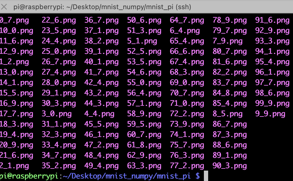
然后需要自己在dataset里导出一些图片：我保存在了mnist_pi文件夹下,“_”后面的是标签，主要是在pc端导出保存到树莓派下

在树莓派上实现numpy的conv2d卷积神经网络做图像分类，加载pytorch的模型参数，推理mnist手写数字识别，并使用多进程加速

树莓派推理端的代码，需要numpy手动重新搭建网络，并且需要手动实现conv2d卷积神经网络和maxpool2d最大池化，然后加载那些保存的矩阵参数，做矩阵乘法和加法

import numpy as np
import os
from PIL import Image

def conv2d(input, weight, bias, stride=1, padding=0):
    batch_size, in_channels, in_height, in_width = input.shape
    out_channels, in_channels, kernel_size, _ = weight.shape

    # 计算输出特征图的大小
    out_height = (in_height + 2 * padding - kernel_size) // stride + 1
    out_width = (in_width + 2 * padding - kernel_size) // stride + 1

    # 添加padding
    padded_input = np.pad(input, ((0, 0), (0, 0), (padding, padding), (padding, padding)), mode='constant')

    # 初始化输出特征图
    output = np.zeros((batch_size, out_channels, out_height, out_width))

    # 执行卷积操作
    for b in range(batch_size):
        for c_out in range(out_channels):
            for h_out in range(out_height):
                for w_out in range(out_width):
                    h_start = h_out * stride
                    h_end = h_start + kernel_size
                    w_start = w_out * stride
                    w_end = w_start + kernel_size

                    # 提取对应位置的输入图像区域
                    input_region = padded_input[b, :, h_start:h_end, w_start:w_end]

                    # 计算卷积结果
                    x = input_region * weight[c_out]
                    bia = bias[c_out]
                    conv_result = np.sum(x, axis=(0,1, 2)) + bia

                    # 将卷积结果存储到输出特征图中
                    output[b, c_out, h_out, w_out] = conv_result

    return output

def max_pool2d(input, kernel_size, stride=None, padding=0):
    batch_size, channels, in_height, in_width = input.shape

    if stride is None:
        stride = kernel_size

    out_height = (in_height - kernel_size + 2 * padding) // stride + 1
    out_width = (in_width - kernel_size + 2 * padding) // stride + 1

    padded_input = np.pad(input, ((0, 0), (0, 0), (padding, padding), (padding, padding)), mode='constant')

    output = np.zeros((batch_size, channels, out_height, out_width))

    for b in range(batch_size):
        for c in range(channels):
            for h_out in range(out_height):
                for w_out in range(out_width):
                    h_start = h_out * stride
                    h_end = h_start + kernel_size
                    w_start = w_out * stride
                    w_end = w_start + kernel_size

                    input_region = padded_input[b, c, h_start:h_end, w_start:w_end]

                    output[b, c, h_out, w_out] = np.max(input_region)

    return output


# 加载保存的模型数据
model_data = np.load('model.npz')

# 提取模型参数
conv_weight = model_data['conv1.weight']
conv_bias = model_data['conv1.bias']
fc_weight = model_data['fc.weight']
fc_bias = model_data['fc.bias']

# 进行推理
def inference(images):
    # 执行卷积操作
    conv_output = conv2d(images, conv_weight, conv_bias, stride=1, padding=0)
    conv_output = np.maximum(conv_output, 0)  # ReLU激活函数
    #maxpool2d
    pool = max_pool2d(conv_output,2)
    # 执行全连接操作
    flattened = pool.reshape(pool.shape[0], -1)
    fc_output = np.dot(flattened, fc_weight.T) + fc_bias
    fc_output = np.maximum(fc_output, 0)  # ReLU激活函数

    # 获取预测结果
    predictions = np.argmax(fc_output, axis=1)

    return predictions


folder_path = './mnist_pi'  # 替换为图片所在的文件夹路径
def infer_images_in_folder(folder_path):
    for file_name in os.listdir(folder_path):
        file_path = os.path.join(folder_path, file_name)
        if os.path.isfile(file_path) and file_name.endswith(('.jpg', '.jpeg', '.png')):
            image = Image.open(file_path)
            label = file_name.split(".")[0].split("_")[1]
            image = np.array(image)/255.0
            image = np.expand_dims(image,axis=0)
            image = np.expand_dims(image,axis=0)
            print("file_path:",file_path,"img size:",image.shape,"label:",label)
            predicted_class = inference(image)
            print('Predicted class:', predicted_class)

infer_images_in_folder(folder_path)

文章来源地址https://www.toymoban.com/news/detail-464769.html

这代码完全就是numpy推理，不需要安装pytorch，树莓派也装不动pytorch，太重了，下面是推理结果，比之前的MLP网络慢很多，主要是手动实现的卷积网络全靠循环实现。

在树莓派上实现numpy的conv2d卷积神经网络做图像分类，加载pytorch的模型参数，推理mnist手写数字识别，并使用多进程加速

conv2d和max_pool2d加速程序：

import numpy as np
import os
from PIL import Image


def conv2d(images,weight,bias,stride=1,padding=1):
    # 卷积操作
    N, C, H, W = images.shape
    F, _, HH, WW = weight.shape
    # 计算卷积后的输出尺寸
    H_out = (H - HH + 2 * padding) // stride + 1
    W_out = (W - WW + 2 * padding) // stride + 1
    # 初始化卷积层输出
    out = np.zeros((N, F, H_out, W_out))
    # 执行卷积运算
    for i in range(H_out):
        for j in range(W_out):
            # 提取当前卷积窗口
            window = images[:, :, i * stride:i * stride + HH, j * stride:j * stride + WW]
            # 执行卷积运算
            out[:, :, i, j] = np.sum(window * weight, axis=(1, 2, 3)) + bias
    # 输出结果
    # print("卷积层输出尺寸:", out.shape)
    return out


import numpy as np

def max_pool2d(input, kernel_size, stride=None, padding=0):
    # 输入尺寸
    batch_size,num_channels, input_height, input_width = input.shape

    # 默认stride等于kernel_size
    if stride is None:
        stride = kernel_size

    # 输出尺寸
    output_height = (input_height - kernel_size + 2 * padding) // stride + 1
    output_width = (input_width - kernel_size + 2 * padding) // stride + 1

    # 添加padding
    if padding > 0:
        padded_input = np.pad(input, [(0, 0), (padding, padding), (padding, padding), (0, 0)], mode='constant')
    else:
        padded_input = input

    # 用于存储输出特征图
    output = np.zeros((batch_size,num_channels, output_height, output_width))

    # 执行最大池化操作
    for i in range(output_height):
        for j in range(output_width):
            start_i = i * stride
            start_j = j * stride
            end_i = start_i + kernel_size
            end_j = start_j + kernel_size
            sub_future = padded_input[:,:, start_i:end_i, start_j:end_j]
            output[:, :,i, j] = np.max(sub_future, axis=(2,3))

    return output


# 加载保存的模型数据
model_data = np.load('conv2d_model.npz')
# 提取模型参数
conv_weight = model_data['conv1.weight']
conv_bias = model_data['conv1.bias']
fc_weight = model_data['fc.weight']
fc_bias = model_data['fc.bias']


# 进行推理
def inference(images):
    # 执行卷积操作
    conv_output = conv2d(images, conv_weight, conv_bias, stride=1, padding=0)
    conv_output = np.maximum(conv_output, 0)  # ReLU激活函数
    #maxpool2d
    pool = max_pool2d(conv_output,2)
    # 执行全连接操作
    flattened = pool.reshape(pool.shape[0], -1)
    fc_output = np.dot(flattened, fc_weight.T) + fc_bias
    fc_output = np.maximum(fc_output, 0)  # ReLU激活函数

    # 获取预测结果
    predictions = np.argmax(fc_output, axis=1)

    return predictions



def infer_images_in_folder(folder_path):
    for file_name in os.listdir(folder_path):
        file_path = os.path.join(folder_path, file_name)
        if os.path.isfile(file_path) and file_name.endswith(('.jpg', '.jpeg', '.png')):
            image = Image.open(file_path)
            label = file_name.split(".")[0].split("_")[1]
            image = np.array(image)/255.0
            image = np.expand_dims(image,axis=0)
            image = np.expand_dims(image,axis=0)
            print("file_path:",file_path,"img size:",image.shape,"label:",label)
            predicted_class = inference(image)
            print('Predicted class:', predicted_class)




if __name__ == "__main__":

    # conv2d(X,weight,b)
    folder_path = './mnist_pi'  # 替换为图片所在的文件夹路径
    infer_images_in_folder(folder_path)

那我们给它加加速吧，下面是一个多线程加速程序：

import numpy as np
import os
from PIL import Image
from multiprocessing import Pool

def conv2d(input, weight, bias, stride=1, padding=0):
    batch_size, in_channels, in_height, in_width = input.shape
    out_channels, in_channels, kernel_size, _ = weight.shape

    # 计算输出特征图的大小
    out_height = (in_height + 2 * padding - kernel_size) // stride + 1
    out_width = (in_width + 2 * padding - kernel_size) // stride + 1

    # 添加padding
    padded_input = np.pad(input, ((0, 0), (0, 0), (padding, padding), (padding, padding)), mode='constant')

    # 初始化输出特征图
    output = np.zeros((batch_size, out_channels, out_height, out_width))

    # 执行卷积操作
    for b in range(batch_size):
        for c_out in range(out_channels):
            for h_out in range(out_height):
                for w_out in range(out_width):
                    h_start = h_out * stride
                    h_end = h_start + kernel_size
                    w_start = w_out * stride
                    w_end = w_start + kernel_size

                    # 提取对应位置的输入图像区域
                    input_region = padded_input[b, :, h_start:h_end, w_start:w_end]

                    # 计算卷积结果
                    x = input_region * weight[c_out]
                    bia = bias[c_out]
                    conv_result = np.sum(x, axis=(0,1, 2)) + bia

                    # 将卷积结果存储到输出特征图中
                    output[b, c_out, h_out, w_out] = conv_result

    return output

def max_pool2d(input, kernel_size, stride=None, padding=0):
    batch_size, channels, in_height, in_width = input.shape

    if stride is None:
        stride = kernel_size

    out_height = (in_height - kernel_size + 2 * padding) // stride + 1
    out_width = (in_width - kernel_size + 2 * padding) // stride + 1

    padded_input = np.pad(input, ((0, 0), (0, 0), (padding, padding), (padding, padding)), mode='constant')

    output = np.zeros((batch_size, channels, out_height, out_width))

    for b in range(batch_size):
        for c in range(channels):
            for h_out in range(out_height):
                for w_out in range(out_width):
                    h_start = h_out * stride
                    h_end = h_start + kernel_size
                    w_start = w_out * stride
                    w_end = w_start + kernel_size

                    input_region = padded_input[b, c, h_start:h_end, w_start:w_end]

                    output[b, c, h_out, w_out] = np.max(input_region)

    return output

# 加载保存的模型数据
model_data = np.load('model.npz')

# 提取模型参数
conv_weight = model_data['conv1.weight']
conv_bias = model_data['conv1.bias']
fc_weight = model_data['fc.weight']
fc_bias = model_data['fc.bias']

# 进行推理
def inference(images):
    # 执行卷积操作
    conv_output = conv2d(images, conv_weight, conv_bias, stride=1, padding=0)
    conv_output = np.maximum(conv_output, 0)  # ReLU激活函数
    # maxpool2d
    pool = max_pool2d(conv_output, 2)
    # 执行全连接操作
    flattened = pool.reshape(pool.shape[0], -1)
    fc_output = np.dot(flattened, fc_weight.T) + fc_bias
    fc_output = np.maximum(fc_output, 0)  # ReLU激活函数

    # 获取预测结果
    predictions = np.argmax(fc_output, axis=1)

    return predictions

labels = []
preds = []
def infer_image(file_path):
    image = Image.open(file_path)
    label = file_path.split("/")[-1].split(".")[0].split("_")[1]
    image = np.array(image) / 255.0
    image = np.expand_dims(image, axis=0)
    image = np.expand_dims(image, axis=0)
    print("file_path:", file_path, "img size:", image.shape, "label:", label)
    predicted_class = inference(image)
    print('Predicted class:', predicted_class)


folder_path = './mnist_pi'  # 替换为图片所在的文件夹路径
pool = Pool(processes=4)  # 设置进程数为2，可以根据需要进行调整

def infer_images_in_folder(folder_path):
    for file_name in os.listdir(folder_path):
        file_path = os.path.join(folder_path, file_name)
        if os.path.isfile(file_path) and file_name.endswith(('.jpg', '.jpeg', '.png')):
            pool.apply_async(infer_image, args=(file_path,))

    pool.close()
    pool.join()


infer_images_in_folder(folder_path)

下图可以看出来，我的树莓派3b+，cpu直接拉满，速度提升4倍：

在树莓派上实现numpy的conv2d卷积神经网络做图像分类，加载pytorch的模型参数，推理mnist手写数字识别，并使用多进程加速

改了一个轻量级的卷积和maxpool的实现，然后再使用多进程加速，可以明显看到cpu的占用率更低了，下次争取把量化后的模型拿过来用

import numpy as np
import os
from PIL import Image
from multiprocessing import Pool


def conv2d(images,weight,bias,stride=1,padding=1):
    # 卷积操作
    N, C, H, W = images.shape
    F, _, HH, WW = weight.shape
    # 计算卷积后的输出尺寸
    H_out = (H - HH + 2 * padding) // stride + 1
    W_out = (W - WW + 2 * padding) // stride + 1
    # 初始化卷积层输出
    out = np.zeros((N, F, H_out, W_out))
    # 执行卷积运算
    for i in range(H_out):
        for j in range(W_out):
            # 提取当前卷积窗口
            window = images[:, :, i * stride:i * stride + HH, j * stride:j * stride + WW]
            # 执行卷积运算
            out[:, :, i, j] = np.sum(window * weight, axis=(1, 2, 3)) + bias
    # 输出结果
    # print("卷积层输出尺寸:", out.shape)
    return out


import numpy as np

def max_pool2d(input, kernel_size, stride=None, padding=0):
    # 输入尺寸
    batch_size,num_channels, input_height, input_width = input.shape

    # 默认stride等于kernel_size
    if stride is None:
        stride = kernel_size

    # 输出尺寸
    output_height = (input_height - kernel_size + 2 * padding) // stride + 1
    output_width = (input_width - kernel_size + 2 * padding) // stride + 1

    # 添加padding
    if padding > 0:
        padded_input = np.pad(input, [(0, 0), (padding, padding), (padding, padding), (0, 0)], mode='constant')
    else:
        padded_input = input

    # 用于存储输出特征图
    output = np.zeros((batch_size,num_channels, output_height, output_width))

    # 执行最大池化操作
    for i in range(output_height):
        for j in range(output_width):
            start_i = i * stride
            start_j = j * stride
            end_i = start_i + kernel_size
            end_j = start_j + kernel_size
            sub_future = padded_input[:,:, start_i:end_i, start_j:end_j]
            output[:, :,i, j] = np.max(sub_future, axis=(2,3))

    return output


# 加载保存的模型数据
model_data = np.load('conv2d_model.npz')
# 提取模型参数
conv_weight = model_data['conv1.weight']
conv_bias = model_data['conv1.bias']
fc_weight = model_data['fc.weight']
fc_bias = model_data['fc.bias']


# 进行推理
def inference(images):
    # 执行卷积操作
    conv_output = conv2d(images, conv_weight, conv_bias, stride=1, padding=0)
    conv_output = np.maximum(conv_output, 0)  # ReLU激活函数
    #maxpool2d
    pool = max_pool2d(conv_output,2)
    # 执行全连接操作
    flattened = pool.reshape(pool.shape[0], -1)
    fc_output = np.dot(flattened, fc_weight.T) + fc_bias
    fc_output = np.maximum(fc_output, 0)  # ReLU激活函数

    # 获取预测结果
    predictions = np.argmax(fc_output, axis=1)

    return predictions



# def infer_images_in_folder(folder_path):
#     for file_name in os.listdir(folder_path):
#         file_path = os.path.join(folder_path, file_name)
#         if os.path.isfile(file_path) and file_name.endswith(('.jpg', '.jpeg', '.png')):
#             image = Image.open(file_path)
#             label = file_name.split(".")[0].split("_")[1]
#             image = np.array(image)/255.0
#             image = np.expand_dims(image,axis=0)
#             image = np.expand_dims(image,axis=0)
#             print("file_path:",file_path,"img size:",image.shape,"label:",label)
#             predicted_class = inference(image)
#             print('Predicted class:', predicted_class)

def infer_image(file_path):
    image = Image.open(file_path)
    label = file_path.split("/")[-1].split(".")[0].split("_")[1]
    image = np.array(image) / 255.0
    image = np.expand_dims(image, axis=0)
    image = np.expand_dims(image, axis=0)
    predicted_class = inference(image)
    print("file_path:", file_path, "img size:", image.shape, "label:", label,'Predicted class:', predicted_class)


def infer_images_in_folder(folder_path):

    while True:
        pool = Pool(processes=4)  # 设置进程数为2，可以根据需要进行调整
        for file_name in os.listdir(folder_path):
            file_path = os.path.join(folder_path, file_name)
            if os.path.isfile(file_path) and file_name.endswith(('.jpg', '.jpeg', '.png')):
                pool.apply_async(infer_image, args=(file_path,))

        pool.close()
        pool.join()



if __name__ == "__main__":

    # conv2d(X,weight,b)
    folder_path = './mnist_pi'  # 替换为图片所在的文件夹路径

    
    infer_images_in_folder(folder_path)