1 可选实验室: 多变量线性回归
在这个实验室中,您将扩展数据结构和以前开发的例程,以支持多个特性。一些程序被更新使得实验室看起来很长,但是它对以前的程序做了一些小的调整使得它可以很快的回顾。
2 目标
扩展我们的回归模型例程以支持多个特性
- 扩展数据结构以支持多个特性
- 重写预测,成本和梯度例程,以支持多个功能
- 利用 NumPy np.dot 向量化它们的实现,以提高速度和简单性
在这个实验室里,我们将利用:
- NumPy,一个流行的科学计算图书馆
- Matplotlib,一个用于绘制数据的流行库
以下是将遇到的一些符号的摘要:

3 问题陈述
您将使用房价预测的激励例子。培训数据集包含三个示例,四个特征(大小、卧室、楼层和年龄)如下表所示。请注意,与早期的实验室不同,大小是平方英尺而不是1000平方英尺。这会导致一个问题,你将在下一个实验室解决!

你将使用这些值建立一个线性回归模型,这样你就可以预测其他房子的价格。例如,一个房子有1200平方英尺,3个卧室,1层,40年。
3.1 矩阵X
先来创建X_ train 和 y _ train 变量。
import copy, math
import numpy as np
import matplotlib.pyplot as plt
plt.style.use('./deeplearning.mplstyle')
np.set_printoptions(precision=2)  # reduced display precision on numpy arrays
X_train = np.array([[2104, 5, 1, 45], [1416, 3, 2, 40], [852, 2, 1, 35]])
y_train = np.array([460, 232, 178])
# data is stored in numpy array/matrix
print(f"X Shape: {X_train.shape}, X Type:{type(X_train)})")
print(X_train)
print(f"y Shape: {y_train.shape}, y Type:{type(y_train)})")
print(y_train)
与上表类似,示例存储在 NumPy 矩阵 X _ train 中。矩阵的每一行代表一个示例。当你有 m 个训练例子(在我们的例子中,m 是3个) ,并且有 n 个特征(在我们的例子中是4个) ,X 是一个带维度的矩阵(m,n)(m 行,n 列)。
输出为:
X Shape: (3, 4), X Type:<class 'numpy.ndarray'>)
[[2104    5    1   45]
 [1416    3    2   40]
 [ 852    2    1   35]]
y Shape: (3,), y Type:<class 'numpy.ndarray'>)
[460 232 178]
3.2 参数向量w,b
w是一个有 n 个元素的向量。每个元素包含与一个特性相关联的参数。在我们的数据集中,n 是4。理论上,我们把它画成一个列向量。
b是一个标量参数。
为了演示,w 和 b 将加载一些接近最优的初始选择值。
b_init = 785.1811367994083
w_init = np.array([ 0.39133535, 18.75376741, -53.36032453, -26.42131618])
print(f"w_init shape: {w_init.shape}, b_init type: {type(b_init)}")
输出:
w_init shape: (4,), b_init type: <class 'float'>
4 多变量模型预测
该模型的多变量预测由线性模型给出:𝑓𝐰,𝑏(𝐱)=𝑤0𝑥0+𝑤1𝑥1+...+𝑤𝑛−1𝑥𝑛−1+𝑏(1)。用向量表示为:𝑓𝐰,𝑏(𝐱)=𝐰⋅𝐱+𝑏(2)。
我们先前的预测将一个特征值乘以一个参数,并添加了一个偏差参数。
我们以前的预测实现的一个直接扩展到多个特征将是实现(1)使用循环每个元素,执行乘法与其参数,然后加入偏差参数在结束。
def predict_single_loop(x, w, b):
    """
    single predict using linear regression

    Args:
      x (ndarray): Shape (n,) example with multiple features
      w (ndarray): Shape (n,) model parameters
      b (scalar):  model parameter

    Returns:
      p (scalar):  prediction
    """
    n = x.shape[0]
    p = 0
    for i in range(n):
        p_i = x[i] * w[i]
        p = p + p_i
    p = p + b
    return p
# get a row from our training data
x_vec = X_train[0,:]
print(f"x_vec shape {x_vec.shape}, x_vec value: {x_vec}")

# make a prediction
f_wb = predict_single_loop(x_vec, w_init, b_init)
print(f"f_wb shape {f_wb.shape}, prediction: {f_wb}")
输出:
x_vec shape (4,), x_vec value: [2104    5    1   45]
f_wb shape (), prediction: 459.9999976194083
注意 x _ vec 的形状。它是一个包含4个元素(4,)的一维NumPy 向量。结果f _ wb 是一个标量。
注意到上面的等式(1)可以用上面的点乘来实现。我们可以利用向量运算来加速预测。回想一下 Python/NumPy 实验室,NumPy np.dot ()[ link ]可以用来执行向量点积。
def predict(x, w, b):
    """
    single predict using linear regression
    Args:
      x (ndarray): Shape (n,) example with multiple features
      w (ndarray): Shape (n,) model parameters
      b (scalar):             model parameter

    Returns:
      p (scalar):  prediction
    """
    p = np.dot(x, w) + b
    return p
# get a row from our training data
x_vec = X_train[0,:]
print(f"x_vec shape {x_vec.shape}, x_vec value: {x_vec}")

# make a prediction
f_wb = predict(x_vec,w_init, b_init)
print(f"f_wb shape {f_wb.shape}, prediction: {f_wb}")
输出:
x_vec shape (4,), x_vec value: [2104    5    1   45]
f_wb shape (), prediction: 459.9999976194082
结果和形状与之前使用循环的版本相同。接下来,np.dot 将用于这些操作。这个预测现在是一个单一的语句。大多数例程将直接实现它,而不是调用单独的预测例程。
5 多变量计算成本
多变量 J (w,b)的成本函数方程是:

其中,

与以前的实验室不同,w 和 x (i)是向量,而不是支持多个特性的标量。下面是公式(3)和(4)的实现。注意,本课程使用了一个标准模式,其中在所有 m 示例上使用了一个 for 循环。
def compute_cost(X, y, w, b):
    """
    compute cost
    Args:
      X (ndarray (m,n)): Data, m examples with n features
      y (ndarray (m,)) : target values
      w (ndarray (n,)) : model parameters
      b (scalar)       : model parameter

    Returns:
      cost (scalar): cost
    """
    m = X.shape[0]
    cost = 0.0
    for i in range(m):
        f_wb_i = np.dot(X[i], w) + b           #(n,)(n,) = scalar (see np.dot)
        cost = cost + (f_wb_i - y[i])**2       #scalar
    cost = cost / (2 * m)                      #scalar
    return cost
# Compute and display cost using our pre-chosen optimal parameters.
cost = compute_cost(X_train, y_train, w_init, b_init)
print(f'Cost at optimal w : {cost}')
输出:
Cost at optimal w : 1.5578904330213735e-12
6 多变量梯度下降法
多变量梯度下降法:

其中,n 是特性的数量,参数 wj,b,同时更新,

m 是数据集中训练例子的数量。fw,b (x (i))是模型的预测值,而 y (i)是目标值。
下面是计算公式(6)和(7)的实现。有很多方法可以实现这一点。
def compute_gradient(X, y, w, b):
    """
    Computes the gradient for linear regression
    Args:
      X (ndarray (m,n)): Data, m examples with n features
      y (ndarray (m,)) : target values
      w (ndarray (n,)) : model parameters
      b (scalar)       : model parameter

    Returns:
      dj_dw (ndarray (n,)): The gradient of the cost w.r.t. the parameters w.
      dj_db (scalar):       The gradient of the cost w.r.t. the parameter b.
    """
    m,n = X.shape           #(number of examples, number of features)
    dj_dw = np.zeros((n,))
    dj_db = 0.

    for i in range(m):
        err = (np.dot(X[i], w) + b) - y[i]
        for j in range(n):
            dj_dw[j] = dj_dw[j] + err * X[i, j]
        dj_db = dj_db + err
    dj_dw = dj_dw / m
    dj_db = dj_db / m

    return dj_db, dj_dw
#Compute and display gradient
tmp_dj_db, tmp_dj_dw = compute_gradient(X_train, y_train, w_init, b_init)
print(f'dj_db at initial w,b: {tmp_dj_db}')
print(f'dj_dw at initial w,b: \n {tmp_dj_dw}')
输出:
dj_db at initial w,b: -1.6739251122999121e-06
dj_dw at initial w,b:
 [-2.73e-03 -6.27e-06 -2.22e-06 -6.92e-05]
def gradient_descent(X, y, w_in, b_in, cost_function, gradient_function, alpha, num_iters):
    """
    Performs batch gradient descent to learn theta. Updates theta by taking
    num_iters gradient steps with learning rate alpha

    Args:
      X (ndarray (m,n))   : Data, m examples with n features
      y (ndarray (m,))    : target values
      w_in (ndarray (n,)) : initial model parameters
      b_in (scalar)       : initial model parameter
      cost_function       : function to compute cost
      gradient_function   : function to compute the gradient
      alpha (float)       : Learning rate
      num_iters (int)     : number of iterations to run gradient descent

    Returns:
      w (ndarray (n,)) : Updated values of parameters
      b (scalar)       : Updated value of parameter
      """

    # An array to store cost J and w's at each iteration primarily for graphing later
    J_history = []
    w = copy.deepcopy(w_in)  #avoid modifying global w within function
    b = b_in

    for i in range(num_iters):

        # Calculate the gradient and update the parameters
        dj_db,dj_dw = gradient_function(X, y, w, b)   ##None

        # Update Parameters using w, b, alpha and gradient
        w = w - alpha * dj_dw               ##None
        b = b - alpha * dj_db               ##None

        # Save cost J at each iteration
        if i<100000:      # prevent resource exhaustion
            J_history.append( cost_function(X, y, w, b))

        # Print cost every at intervals 10 times or as many iterations if < 10
        if i% math.ceil(num_iters / 10) == 0:
            print(f"Iteration {i:4d}: Cost {J_history[-1]:8.2f}   ")

    return w, b, J_history #return final w,b and J history for graphing
# initialize parameters
initial_w = np.zeros_like(w_init)
initial_b = 0.
# some gradient descent settings
iterations = 1000
alpha = 5.0e-7
# run gradient descent
w_final, b_final, J_hist = gradient_descent(X_train, y_train, initial_w, initial_b,
                                                    compute_cost, compute_gradient,
                                                    alpha, iterations)
print(f"b,w found by gradient descent: {b_final:0.2f},{w_final} ")
m,_ = X_train.shape
for i in range(m):
    print(f"prediction: {np.dot(X_train[i], w_final) + b_final:0.2f}, target value: {y_train[i]}")
Iteration 0: Cost 2529.46 Iteration 100: Cost 695.99 Iteration 200: Cost 694.92 Iteration 300: Cost 693.86 Iteration 400: Cost 692.81 Iteration 500: Cost 691.77 Iteration 600: Cost 690.73 Iteration 700: Cost 689.71 Iteration 800: Cost 688.70 Iteration 900: Cost 687.69 b,w found by gradient descent: -0.00,[ 0.2 0. -0.01 -0.07] prediction: 426.19, target value: 460 prediction: 286.17, target value: 232 prediction: 171.47, target value: 178
# plot cost versus iteration
fig, (ax1, ax2) = plt.subplots(1, 2, constrained_layout=True, figsize=(12, 4))
ax1.plot(J_hist)
ax2.plot(100 + np.arange(len(J_hist[100:])), J_hist[100:])
ax1.set_title("Cost vs. iteration");  ax2.set_title("Cost vs. iteration (tail)")
ax1.set_ylabel('Cost')             ;  ax2.set_ylabel('Cost')
ax1.set_xlabel('iteration step')   ;  ax2.set_xlabel('iteration step')
plt.show()
输出:
 文章来源:https://www.toymoban.com/news/detail-562445.html
这些结果一点都不鼓舞人心!成本仍在下降,我们的预测不是很准确。下一个实验室将探讨如何改进这一点。 文章来源地址https://www.toymoban.com/news/detail-562445.html
到了这里,关于吴恩达机器学习2022-Jupyter的文章就介绍完了。如果您还想了解更多内容,请在右上角搜索TOY模板网以前的文章或继续浏览下面的相关文章,希望大家以后多多支持TOY模板网!