Practice Lab: Linear Regression
Exercise 1
Complete the compute_cost below to:
-
Iterate over the training examples, and for each example, compute:
-
The prediction of the model for that example
f w b ( x ( i ) ) = w x ( i ) + b f_{wb}(x^{(i)}) = wx^{(i)} + b fwb(x(i))=wx(i)+b -
The cost for that example c o s t ( i ) = ( f w b − y ( i ) ) 2 cost^{(i)} = (f_{wb} - y^{(i)})^2 cost(i)=(fwb−y(i))2
-
-
Return the total cost over all examples
J ( w , b ) = 1 2 m ∑ i = 0 m − 1 c o s t ( i ) J(\mathbf{w},b) = \frac{1}{2m} \sum\limits_{i = 0}^{m-1} cost^{(i)} J(w,b)=2m1i=0∑m−1cost(i)- Here, m m m is the number of training examples and ∑ \sum ∑ is the summation operator
If you get stuck, you can check out the hints presented after the cell below to help you with the implementation.文章来源地址https://www.toymoban.com/news/detail-709262.html
# UNQ_C1
# GRADED FUNCTION: compute_cost

def compute_cost(x, y, w, b):
    # number of training examples
    m = x.shape[0]
    # You need to return this variable correctly
    total_cost = 0

    ### START CODE HERE ###
    for i in range(m):
        total_cost+=((x[i]*w+b)-y[i])**2
    total_cost=total_cost/(2*m)
    ### END CODE HERE ###

    return total_cost
Exercise 2
Please complete the compute_gradient function to:
-
Iterate over the training examples, and for each example, compute:
-
The prediction of the model for that example
f w b ( x ( i ) ) = w x ( i ) + b f_{wb}(x^{(i)}) = wx^{(i)} + b fwb(x(i))=wx(i)+b -
The gradient for the parameters w , b w, b w,b from that example
∂ J ( w , b ) ∂ b ( i ) = ( f w , b ( x ( i ) ) − y ( i ) ) \frac{\partial J(w,b)}{\partial b}^{(i)} = (f_{w,b}(x^{(i)}) - y^{(i)}) ∂b∂J(w,b)(i)=(fw,b(x(i))−y(i))
∂ J ( w , b ) ∂ w ( i ) = ( f w , b ( x ( i ) ) − y ( i ) ) x ( i ) \frac{\partial J(w,b)}{\partial w}^{(i)} = (f_{w,b}(x^{(i)}) -y^{(i)})x^{(i)} ∂w∂J(w,b)(i)=(fw,b(x(i))−y(i))x(i)
-
-
Return the total gradient update from all the examples
∂ J ( w , b ) ∂ b = 1 m ∑ i = 0 m − 1 ∂ J ( w , b ) ∂ b ( i ) \frac{\partial J(w,b)}{\partial b} = \frac{1}{m} \sum\limits_{i = 0}^{m-1} \frac{\partial J(w,b)}{\partial b}^{(i)} ∂b∂J(w,b)=m1i=0∑m−1∂b∂J(w,b)(i)∂ J ( w , b ) ∂ w = 1 m ∑ i = 0 m − 1 ∂ J ( w , b ) ∂ w ( i ) \frac{\partial J(w,b)}{\partial w} = \frac{1}{m} \sum\limits_{i = 0}^{m-1} \frac{\partial J(w,b)}{\partial w}^{(i)} ∂w∂J(w,b)=m1i=0∑m−1∂w∂J(w,b)(i)文章来源:https://www.toymoban.com/news/detail-709262.html
- Here, m m m is the number of training examples and ∑ \sum ∑ is the summation operator
If you get stuck, you can check out the hints presented after the cell below to help you with the implementation.
# UNQ_C2
# GRADED FUNCTION: compute_gradient
def compute_gradient(x, y, w, b):
    # Number of training examples
    m = x.shape[0]
    # You need to return the following variables correctly
    dj_dw = 0
    dj_db = 0

    ### START CODE HERE ###
    for i in range(m):
        f_wb=w*x[i]+b
        dj_dw_i=(f_wb-y[i])*x[i]
        dj_db_i=f_wb-y[i]
        dj_dw+=dj_dw_i
        dj_db+=dj_db_i
    dj_dw=dj_dw/m
    dj_db=dj_db/m
    ### END CODE HERE ###

    return dj_dw, dj_db
到了这里,关于吴恩达机器学习week2实验答案Practice Lab Linear Regression【C1_W2_Linear_Regression】的文章就介绍完了。如果您还想了解更多内容,请在右上角搜索TOY模板网以前的文章或继续浏览下面的相关文章,希望大家以后多多支持TOY模板网!


