前言
花了好大心血完成了一份留学作业系列——1:电机控制设计;供大家参考,文末有MATLAB程序及无水印Word文档。
1、Overview
Control design is very important in for power electronics, such as the application on converters and motor control. In this lab, we will learn how to design a PI controller for a DC motor to meet the required specifications. The lab will be conducted on the simulation software Matlab Simulink. The design of PI controllers requires background knowledge and theories on both DC machine as well as the control, such as the derivation of transfer functions for motor current and speed, which are presented as supporting documentations and posted on the Canvas. They should be studied before this lab to ensure you can follow up in the lab class.
1.1、Specific objectives
- To understand the process of deriving the model of a control system
- To measure the stability and accuracy of a control loop
- To implement a tuning strategy for a closed loop system (PI controller)
- To check the system operation against the technical specifications
1.2、Resources
Following documents are provided for you to understand and develop the lab section by section:
- Modeling of a dc motor - mod_DC_Motor [1]
- PI analog controllers and first order systems - PI_order1 [2]
These documents can be downloaded from the Canvas site under Module->Laboratory note.
1.3 、Industrial context
In the context of an industrial application, we want to implement a system to control the speed of a dc motor which may drive a conveyor belt that dispatches mechanical parts. The system is controlled by an analog controller operating in the first quadrant. It is supplied through a power converter such as a dc buck converter. With controlling duty cycles of the converter, the supply voltage of the dc motor can be varied, and the speed of the motor can be controlled to meet the load variations.
1.4 、Architecture of the system
The block diagram in Fig 1 (a) illustrates a general control scheme, while the Fig.1 (b) shows the flowchart of the control loops to be used in this lab.
Fig.1 (a) Block diagram of general control loop
For this type of servo mechanical system, the current (and therefore the torque) should be controlled in order to avoid lurching and vibrations that can be destructive for the motor. We will use a classical two-loop structure with one inner loop (current control) and one outer loop (speed control).

Fig.1 (b) Block diagram of control loop for this lab
1.5 、Approach/Steps
After the system is modelled, the simulation tool can be used to analyze the behaviour, to adjust the controllers and to ensure the motor performance.
- Search for variables associated with the operating point by modelling of the motor and the load. In this step, you need to set up a buck converter model and dc motor model in Simulink to conduct open-loop operation.
- Modelling the buck converter and dc motor by using their transfer functions and compare with one modelled by their physical modules.
- Identification of the response signal and adjustment of the current controller. You need to run a Bode plots to work out PI controller (Kp and Ki) for the current to meet the control requirements.
- Identification of the response in terms of speed and adjustment of the controller. You need to run step response to work out PI controller for the speed to meet the control requirements.
- Setting limitations on voltage and current, defined by the field of application.
- Analysis of the results and tests on the real structure with the physical modules of converter and motor.
The steps above will be implemented section by section below.
2、MODELLING THE MOTOR AND THE LOAD
2.1Simulate a DC motor by its physical model
A separately excited dc machine with the constant flux will be used to model a dc motor in Matlab. Fig.2 shows the schematic diagram in Matlab Simulink. Please refer to details in the Tutorial on how to establish an open-loop dc motor control the physical models.
- Fig. 2 Schematic diagram of buck converter and DC motor with a load
The load torque (friction) is proportional to the speed. It can be expressed as Cr = K1Ω, where Ω is the speed and the constant K1 = 0.0005 Nm/(rad/sec). The parameters of the motor are shown in Fig.3
- Fig.3 DC motor parameters
Check the parameters for the models in Fig.2 and enter values for each model. Apart from the motor parameters shown in Fig.3, the rest of parameters for the models in Fig.2 are shown or to be calculated below.
Check the parameters for the models in Fig.2 and enter values for each model. Apart from the motor parameters shown in Fig.3, the rest of parameters for the models in Fig.2 are shown or to be calculated below.
- Buck converter: input voltage Vs=24V, duty cycle is 60.4%, and C=100 uF
- Calculate inductance of Lc of the buck converter to achieve the current ripple less than 5% with the switching frequency of 40 kHz;
- DC motor: the parameters of the motor are shown in Fig.3. In the Simulink block diagram of Fig.2, the field voltage is 24 V. What is the motor armature voltage Va out of the buck converter?
Build and simulate the system shown in Fig.2 and check if you obtain a speed of 1500 rpm in the steady state. Record below the response time at 90 % (Tr) of the final value as well as the armature current (Ia) in the steady state. You may record the waveforms for the lab report. Measure the current ripple and see if it is less than 5%.
- V = 14.1V ; Tr = 61.5ms ; Ia = 1.077A Ia = 18.33mA .
2.2、Modelling the motor / load by its mathematical models (transfer functions)
Fig.4 (a) is the block diagram of the motor transfer functions while the diagram in Fig.4 (b) shows the Simulink blocks based on it. Refer to the resource document mod_DC_Motor [1] to derive the parameters for TF1 and TF2 for the dc motor in Fig.4 (b).
- Fig.4 (a) Block diagram for a motor

- Fig.4 (b) Simulink diagram of the DC motor and buck converter by transfer functions
The value of the friction coefficient for Block TF2 is: f = 5.17 μN*m/(rad/sec). For the TF1 block (check the format of a transfer function in Simulink), the numerator and denominator are: (Note the total inductance in the denominator of TF1 should include both inductors from the armature of the motor as well as the Lc from the buck converter)
- num(s) = 1 ; den(s) = 0.92e-3S+2.85 ;
For the TF2 block :
-
num(s) = 1 ; den(s) = 63.5e-6S+2.17e-6 ;
Enter the parameters for the blocks TF1 and TF2 and use the armature voltage V obtained in Section 2.1 for Va. Build and simulate the circuit shown in Fig.4 (b). Record the speed response and measure values for the parameters below from it. Note the speed shows the speed in the unit of rad/s. -
Tr = 59.69mS ; Ia = 1.053A .
Compare values of Tr and Ia with those from Fig.2 in the section 2.1. What can you conclude?
Load motor can be represented by mathematical model or transfer function. By comparing the mathematical model and transfer function, it can be concluded as follows: under current conditions, the motor load expressed by mathematical equation is the same as that directly used in simulink DC Machine module, and the Tr and Ia values obtained are very close.
3、CONTROL LOOP DESIGN
As shown in Fig.1 (b), two control loops will be designed for the motor control: current control and speed control. You need to study the resource document mod_DC_Motor [1] as well as the PI_order1 [2], to be able to follow up the tasks in this section.
3.1、 Design the Current Control Loop
3.1.1、Identification of the transfer function
Refer to the Resource document mod_DC_Motor [1]. Re-draw the dc motor block diagram in Fig.4 (a) as below, the transfer function of I(s)/Um(s) can be derived.

- Fig.6 The block diagram for current control
The theoretical analysis gives the expression of the transfer function of the current in the open loop circuit:


Use the Matlab file built in Fig.4 (b) to measure the bode plot for the system in Fig.6. To do it, click APPS and then open Model Linearizer as highlighted below.
After open Model Linearizer the window below is popped up for you to run Bode plot.
Before run the Bode plot, first add perturbation to the input voltage Va and take the output from the current. In this case, an input perturbation is added to Va and output measurement is set at the current output Ia, as highlighted in yellow in Fig.7.
- Fig.7 Run Bode plot for the current control transfer function

3.1.2、Calculating the current controller
We will choose a PI type controller with an integration time constant Ti (=Kp/Ki) so that Ti = 1/ω2 (see the asymptotic Bode plot in Section 3.1.1). Moreover, we will set a response time, Tr , at 90 % in a closed loop so that Tr = 1 ms bearing in mind that for a first order system we can estimate that (ω0 = cut-off frequency). Note Ti= Kp/Ki, where Kp and Ki are the proportional and integral gain respectively.
On the Bode diagram obtained in Section 3.1.1 (for the system in Fig.7), locate the frequency ω2 and calculate Ti.
- ω2 =314rad/S ;
Ti = 1/ω2 = 0.00318471337579617834394904458599
Calculate the value of ω0 in order to obtain a response time (Tr) equal to 1 ms.
- ω0 = 3000 rad/S ;
Now build the block diagram in Fig.8 (a) in Simulink, and enter parameters for the PI controller as: Ti = 1/ω2 (so Ki= ω2) and Kp=1. Simulate the open loop circuit in Fig.8(a). Measure the value of the circuit gain at the cut-off frequency 0.
- Fig. 8 (a) PI controller for current control loop
- G(0) = -11.9dB ;
Determine the value of Kp so that achieve a gain of 0 dB at the frequency 0 by G(0)=20*log(Kp).
- Kp = 3.93955 .
- Ki = 1.2357e3 .
- The rise time is 1.82ms, which is greater than 1ms.
With the proportional gain worked out above, the integral gain Ki can be recalculated by Ti=Kp/Ki. These should be the final values for the current PI controller. Confirm your calculations by setting the parameters of the controller again and running the simulation for the system in Fig. 8 (b) in which the current control loop is closed. Observe the step response in the closed loop for the armature current Ia in the time domain and check if the rising time less than 1ms.
- Fig. 8 (b) Step response test for the current control loop
3.2、Designing the speed control loop
In this section we are going to work out a PI controller for the speed control loop.
From the supporting documentation mod_DC_Motor [1], we know the transfer function for the motor speed control in Fig.4 (a) can be derived as equation below with an assumption, which is the first order system.
Then we can use the equations derived in the supporting documentation PI_order1 (showing below as well), to design the Kp and Ki of the speed PI controller.
- Eq.(2.4)

- Eq.(2.3)
The rising time Tr for the speed is expected to be less than 100 ms. To work out Ti we need to find out the time constant of the system first.
3.2.1、Identification in an open loop in the time domain
Build the schematic diagram in Fig.9 in Simulink. Calculate the scaling factor Ktac, so that for Vcons = 5 V, we want to obtain a speed equal to 157 rad/s (=1500 rpm). Note: as mentioned in the section 1.2, the unit of speed derived from the transfer functions is rad/s.
- Ktac = 5/157 =0.03184713375796178343949044585987 .
Run the simulation and observe the signal Vcons (speed reference) and V(speed feedback). Then refer to the resource document PI_order1 [2] and identify the time constant τ, as well as the circuit gain for the loop K (in the steady state). Note these parameters are referred to the ones in the transfer function H(s) in resource document PI_order1 [2].
That is the time constant τ is at 63% of the full scale output value, and the static gain K=V/Vcons.
- τ = 127.571mS ; K = 2.182 .

- Fig.9 Work out the parameters of the first order transfer function of the motor
3.2.2、Designing the speed controller
Determine the parameters A and Ti of the speed PI controller (series) that ensures a response time Tr in a closed loop of approximately 100 ms.
Refer to the Equation (2.3) and (2.4) in resource document PI_order1 [2], plus the time constant τ and the loop gain K from the section 3.2.1, and determine the following parameters
- KB = 6.6543 ; A = 3.0496 ; Ti = 0.0580 ;
Can you please explain your calculations?
According to the following 3 formulas:
Eq.1
Eq.2
Eq.3
And the previous calculated values into formula 1, formula 2, formula 3, using matlab to calculate. The matlab code is as follows:
Tr=100e-3;
TAO=127.571e-3;
K=2.182;
A=(6TAO/Tr-1)/K
Ti=4KATAO/((1+KA)(1+KA))
KB=KA
Build the schematic diagram in Fig.10 to establish the close loop of the speed control. Enter the parameter Ktac, and PI controller for the speed loop. Simulate the circuit. Visualize the speed and conclude on the stability, accuracy, and response time.
- Fig.10 Close loop of speed control
4、COMPLETE CONTROL SYSTEM
4.1、Current limiting
So far you have built the PI controller for the speed and current control. Look at the diagram in Fig.10 and simulate the circuit again in order to visualise the amplitude of the current of the motor.
What is the maximum value of the current in transient state? Ia_max = 12.33A .
The large starting current of the motor can cause damage to the insulation. To limit the maximum current, modify the circuit in Fig.10 to Fig.11 by adding a limiter that limits the current amplitude at 3 A. Then run the simulation again and see the effect of this limitation on armature current Ia. Record the waveform and compare with the one without the limiter. How does this limiter affect the response time of the speed?
As can be seen from the figure window, the response speed of the system is slowed down after the limiter is added.
- Fig.11 Add current limiter in the control loop to cap the maximum current
4.2、Development of the entire system
With the models of different parts of the system, we can study the relationship between different variables, and design the control loops. We are now going to conclude the study by simulating the complete system, as shown in Fig.12. Note the first limiter in Fig.12 is to limit maximum transient current and the second limiter is to limit the reference voltage which can be set to 0 to 6.
- Fig.12 Schematic diagram of current and speed control of DC motor with DC buck converter


You will carry out a test with the change of the speed reference from 1200 rpm to 1800 rpm which correspond to Vcons = 4 V~6 V). In these conditions the motor is operating at its nominal power. The table below shows the settings for the reference speed Vcons.
Run the simulation and observe the speed reference (Vcons), the actual speed (Speed), and the armature current as well as other parameters of interest. Record the response waveforms and identify the specifications of the control loop are met or not.
Comment on the speed waveform with reference to the target speed Vcons and identify the problem.

Running the simulation, it can be seen that with the change of the reference speed Vcons, the speed of the motor also changes with the same trend. And the response speed is fast. When the Vcons input is 4V, the motor speed output is 1200rpm. When the Vcons input is 6V, the motor speed output is 1800rpm. However, the motor has inertia, and the response of inertia cannot be eliminated, and it takes about 700ms from 1800rpm to 0rpm.
Reference
[1] Modeling of a dc motor - mod_DC_Motor , on Canvas of UoS
[2] PI analog controllers and first order systems - PI_order1, on Canvas of UoS
5、工程及文档获取
下载链接:https://download.csdn.net/download/weixin_46423500/88347742
MATLAB:电机控制(Motor Control)
其中,zz为最终程序,gc为过程程序供大家参考。 文章来源:https://www.toymoban.com/news/detail-733116.html
 文章来源地址https://www.toymoban.com/news/detail-733116.html
到了这里,关于MATLAB:电机控制(Motor Control)的文章就介绍完了。如果您还想了解更多内容,请在右上角搜索TOY模板网以前的文章或继续浏览下面的相关文章,希望大家以后多多支持TOY模板网!