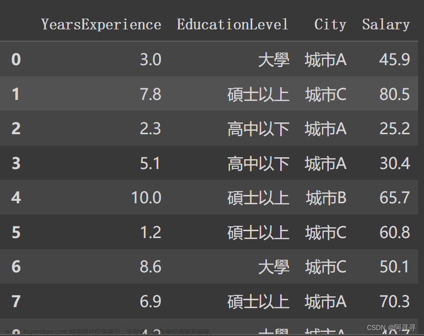
比如你做了一个企业想要招人,但是不知道月薪应该定在多少,你做了一个月薪和收入的调研,包括年限、学历、地区和月薪
做一个月薪=w1年限+w2学历+w3*城市+…+b的工作年限和薪资的多元线性模型,然后找出最适合线性模型的直线-成本函数、梯度下降方式,来预估你可以每个月给员工发薪资是的多少
一、导入数据
# 导入数据
import pandas as pd

url = "https://raw.githubusercontent.com/GrandmaCan/ML/main/Resgression/Salary_Data2.csv"
data = pd.read_csv(url)
data

# # y = w*x + b
# x = data["YearsExperience"]
# y = data["Salary"]
结果
二、资料预处理:label-encoding、one hot encoding
将学历和城市转化成特征
学历:高中以下 :0
大学:1
硕士以上:2
城市:one hot encoding 从一个特征转换成多个特征,把城市转换为3个特征,但是过多的特征很浪费运算,我们这里可以换成CityA、CityB、CityC,然后CityC可以从前两城市推算出来,所以可以只留下来CityA、CityB
data["EducationLevel"] = data["EducationLevel"].map({"高中以下":0,"大學":1,"碩士以上":2})
data
结果

# OneHotEncoder 城市特征转换
from sklearn.preprocessing import OneHotEncoder # sklearn套件

onehot_encoder = OneHotEncoder()
onehot_encoder.fit(data[["City"]])
city_encoded = onehot_encoder.transform(data[["City"]]).toarray()
city_encoded
data[["CityA","CityB","CityC"]] = city_encoded
data = data.drop(["City","CityC"],axis=1) # 去掉城市C
data

三、资料与处理:train 、test 训练集-测试集分组
,训练集用来找最佳斜率w/b,测试集用来测试最佳斜率
from sklearn.model_selection import train_test_split

x = data[["YearsExperience","EducationLevel","CityA","CityB"]]
y = data["Salary"]

x_train,x_test,y_train,y_test = train_test_split(x,y,test_size=0.2,random_state=87)
# len(x),len(x_train),len(x_test)
x_train = x_train.to_numpy()
x_test = x_test.to_numpy()
y_train = y_train.to_numpy()
y_test = y_test.to_numpy()
x_train
结果
array([[ 4.6,  1. ,  1. ,  0. ],
       [ 4.3,  1. ,  1. ,  0. ],
       [ 6.1,  2. ,  1. ,  0. ],
       [ 3.6,  1. ,  1. ,  0. ],
       [ 6.3,  2. ,  1. ,  0. ],
       [ 4.8,  1. ,  1. ,  0. ],
       [ 7.2,  2. ,  0. ,  0. ],
       [10. ,  2. ,  0. ,  1. ],
       [ 1.8,  2. ,  0. ,  0. ],
       [ 2.1,  0. ,  1. ,  0. ],
       [ 3.9,  1. ,  1. ,  0. ],
       [ 7.6,  2. ,  0. ,  0. ],
       [10. ,  2. ,  0. ,  1. ],
       [ 8.2,  1. ,  0. ,  0. ],
       [ 5.1,  0. ,  1. ,  0. ],
       [10. ,  2. ,  0. ,  1. ],
       [ 4.2,  1. ,  1. ,  0. ],
       [ 5.3,  0. ,  1. ,  0. ],
       [ 1.5,  2. ,  0. ,  0. ],
       [ 7.4,  2. ,  0. ,  0. ],
       [ 5. ,  0. ,  1. ,  0. ],
       [ 2.4,  0. ,  1. ,  0. ],
       [ 3. ,  1. ,  1. ,  0. ],
       [ 5.2,  0. ,  1. ,  0. ],
       [ 8. ,  1. ,  0. ,  0. ],
       [ 8.6,  1. ,  0. ,  0. ],
       [ 8.4,  1. ,  0. ,  0. ],
       [10. ,  2. ,  0. ,  1. ]])
四、做特征缩放 Feature Scaling,加速gradient descen
目的让特征大小范围接近,加速gradient descent
特征参数:标准化公式:
(x - mean(x))/ x标准差
from sklearn.preprocessing import StandardScaler
scaler = StandardScaler()
scaler.fit(x_train) #看训练集的资料 标准化公式
x_train = scaler.transform(x_train) #转换结果直接替换掉

x_test = scaler.transform(x_test)
五、预测值公式:y_pred=w1x1 + w2x2 +w3x3 +w4x4 +b
import numpy as np
# y=w1*x1 + w2*x2 +w3*x3 +w4*x4 +b
w = np.array([1,2,3,4])
b = 1
y_pred = (x_train * w).sum(axis=1) + b
y_pred
结果
array([10.6, 10.3, 14.1,  9.6, 14.3, 10.8, 12.2, 19. ,  6.8,  6.1,  9.9,
       12.6, 19. , 11.2,  9.1, 19. , 10.2,  9.3,  6.5, 12.4,  9. ,  6.4,
        9. ,  9.2, 11. , 11.6, 11.4, 19. ])
[71]
0 秒
六、cost_function 价值函数:找一条最适合的曲线
公式:月薪 = w1年限 + w2学历 + w3CityA + w4CityB + b
cost = (真是数据-预测值)**2/取平均
((y_train-y_pred)**2).mean() #(真是数据-预测值)**2/取平均
结果
1772.9485714285713
def compute_cost(x,y,w,b):
  y_pred = (x * w).sum(axis=1) + b
  cost = ((y-y_pred)**2).mean()
  return cost
w = np.array([1,2,3,4])
b = 0
compute_cost(x_train,y_train,w,b)
结果
1853.0200000000002
七、设定optimizer gradient-descent 梯度下降函数:根据斜率改变参数
找出最好的w和b
5个参数:
w1 - w1方向斜率学习率 -->求微分后 --> w1方向斜率 = 2x1(y_pred-y)
w2 - w2方向斜率学习率 -->求微分后 --> w2方向斜率 = 2x2(y_pred-y)
w3 - w3方向斜率学习率 -->求微分后 --> w3方向斜率 = 2x3(y_pred-y)
w4 - w4方向斜率学习率 -->求微分后 --> w4方向斜率 = 2x4(y_pred-y)
b - b方向斜率学习率 -->求微分后 --> b方向斜率 = 2(y_pred-y)
y_pred = (x_train * w).sum(axis=1) + b
b_gradient = (y_pred-y_train).mean()
w_gradient = np.zeros(x_train.shape[1])
#w_gradient
for i in range(x_train.shape[1]):
  w_gradient[i] = (x_train[:,i]*(y_pred-y_train)).mean()
w_gradient,b_gradient

# w1_gradient = (x_train[:,0]*(y_pred-y_train)).mean()
# w2_gradient = (x_train[:,1]*(y_pred-y_train)).mean()
# w3_gradient = (x_train[:,2]*(y_pred-y_train)).mean()
# w4_gradient = (x_train[:,3]*(y_pred-y_train)).mean()
# b_gradient,w1_gradient,w2_gradient,w3_gradient,w4_gradient
结果
array([-252.14928571, -57.51428571, -16.93928571, -6.72857143])
# 定义梯度下降函数
def compute_gradient(x,y,w,b):
  y_pred = (x * w).sum(axis=1) + b
  b_gradient = (y_pred-y).mean() # 计算b方向的额斜率
  w_gradient = np.zeros(x.shape[1]) #创建一个0的矩阵
  #w_gradient
  for i in range(x.shape[1]):
    w_gradient[i] = (x[:,i]*(y_pred-y)).mean() # 计算每个w方向的额斜率
  return w_gradient,b_gradient
w = np.array([1,2,2,4])
b = 1
learning_rate=0.001
w_gradient,b_gradient = compute_gradient(x_train,y_train,w,b)
print(compute_cost(x_train,y_train,w,b))
w = w - w_gradient*learning_rate
b = b - b_gradient*learning_rate
#w,b
print(compute_cost(x_train,y_train,w,b))
np.set_printoptions(formatter={'float':'{:.2e}'.format})
def gradient_descent(x, y, w_init, b_init, learning_rate, cost_function, gradient_function, run_inter, p_inter=1000):
  c_his = []
  b_his = []
  w_his = []

  w = w_init
  b = b_init

  for i in range(run_inter):
    w_gradient,b_gradient = gradient_function(x,y,w,b)
    w = w-w_gradient*learning_rate
    b = b-b_gradient*learning_rate
    cost = cost_function(x,y,w,b)
    c_his.append(cost)
    b_his.append(b)
    w_his.append(w)
    #w,b
    if i%p_inter == 0:
      print(f"Ieration {i:5}: cost {cost:.4e}, w: {w:}, b: {b:.4e}, w_gradient: {w_gradient:}, b_gradient: {b_gradient:.4e}")

  return w,b,w_his,b_his,c_his
# 找到最合适的w,b
w_init = np.array([1,2,2,4])
b_init = 0
learning_rate = 1.0e-3
run_inter = 10000
w_final,b_final,w_his,b_his,c_his = gradient_descent(x_train, y_train, w_init, b_init, learning_rate, compute_cost, compute_gradient, run_inter, p_inter=1000)
结果
Ieration     0: cost 2.8048e+03, w: [1.01e+00 2.01e+00 1.99e+00 4.00e+00], b: 5.0950e-02, w_gradient: [-5.35e+00 -1.22e+01 9.62e+00 -1.12e+00], b_gradient: -5.0950e+01
Ieration  1000: cost 4.0918e+02, w: [2.38e+00 8.45e+00 -2.10e+00 2.17e+00], b: 3.2235e+01, w_gradient: [9.88e-02 -3.40e+00 1.41e+00 2.59e+00], b_gradient: -1.8734e+01
Ieration  2000: cost 8.4076e+01, w: [2.28e+00 1.08e+01 -2.79e+00 4.25e-03], b: 4.4068e+01, w_gradient: [7.85e-03 -1.62e+00 2.54e-01 1.70e+00], b_gradient: -6.8884e+00
Ieration  3000: cost 3.6451e+01, w: [2.38e+00 1.20e+01 -2.85e+00 -1.32e+00], b: 4.8420e+01, w_gradient: [-1.89e-01 -9.01e-01 -6.39e-02 1.01e+00], b_gradient: -2.5328e+00
Ieration  4000: cost 2.8488e+01, w: [2.61e+00 1.27e+01 -2.73e+00 -2.11e+00], b: 5.0020e+01, w_gradient: [-2.55e-01 -5.36e-01 -1.71e-01 6.17e-01], b_gradient: -9.3132e-01
Ieration  5000: cost 2.6669e+01, w: [2.87e+00 1.31e+01 -2.54e+00 -2.61e+00], b: 5.0608e+01, w_gradient: [-2.52e-01 -3.37e-01 -1.94e-01 3.95e-01], b_gradient: -3.4244e-01
Ieration  6000: cost 2.6016e+01, w: [3.10e+00 1.34e+01 -2.35e+00 -2.93e+00], b: 5.0824e+01, w_gradient: [-2.23e-01 -2.23e-01 -1.82e-01 2.64e-01], b_gradient: -1.2591e-01
Ieration  7000: cost 2.5691e+01, w: [3.31e+00 1.36e+01 -2.18e+00 -3.15e+00], b: 5.0904e+01, w_gradient: [-1.87e-01 -1.55e-01 -1.58e-01 1.84e-01], b_gradient: -4.6298e-02
Ieration  8000: cost 2.5505e+01, w: [3.48e+00 1.37e+01 -2.04e+00 -3.31e+00], b: 5.0933e+01, w_gradient: [-1.52e-01 -1.12e-01 -1.32e-01 1.32e-01], b_gradient: -1.7024e-02
Ieration  9000: cost 2.5394e+01, w: [3.61e+00 1.38e+01 -1.92e+00 -3.42e+00], b: 5.0944e+01, w_gradient: [-1.22e-01 -8.29e-02 -1.07e-01 9.72e-02], b_gradient: -6.2595e-03
Ieration 10000: cost 2.5327e+01, w: [3.72e+00 1.39e+01 -1.82e+00 -3.51e+00], b: 5.0948e+01, w_gradient: [-9.63e-02 -6.27e-02 -8.62e-02 7.28e-02], b_gradient: -2.3016e-03
Ieration 11000: cost 2.5286e+01, w: [3.81e+00 1.40e+01 -1.74e+00 -3.57e+00], b: 5.0949e+01, w_gradient: [-7.59e-02 -4.80e-02 -6.85e-02 5.53e-02], b_gradient: -8.4628e-04
Ieration 12000: cost 2.5261e+01, w: [3.88e+00 1.40e+01 -1.68e+00 -3.62e+00], b: 5.0950e+01, w_gradient: [-5.95e-02 -3.71e-02 -5.42e-02 4.23e-02], b_gradient: -3.1117e-04
Ieration 13000: cost 2.5246e+01, w: [3.93e+00 1.40e+01 -1.63e+00 -3.65e+00], b: 5.0950e+01, w_gradient: [-4.66e-02 -2.88e-02 -4.27e-02 3.26e-02], b_gradient: -1.1442e-04
Ieration 14000: cost 2.5237e+01, w: [3.97e+00 1.41e+01 -1.60e+00 -3.68e+00], b: 5.0950e+01, w_gradient: [-3.65e-02 -2.25e-02 -3.36e-02 2.53e-02], b_gradient: -4.2071e-05
Ieration 15000: cost 2.5231e+01, w: [4.00e+00 1.41e+01 -1.57e+00 -3.71e+00], b: 5.0950e+01, w_gradient: [-2.85e-02 -1.75e-02 -2.64e-02 1.96e-02], b_gradient: -1.5469e-05
Ieration 16000: cost 2.5227e+01, w: [4.03e+00 1.41e+01 -1.54e+00 -3.72e+00], b: 5.0950e+01, w_gradient: [-2.23e-02 -1.37e-02 -2.07e-02 1.52e-02], b_gradient: -5.6880e-06
Ieration 17000: cost 2.5225e+01, w: [4.05e+00 1.41e+01 -1.52e+00 -3.74e+00], b: 5.0950e+01, w_gradient: [-1.74e-02 -1.07e-02 -1.62e-02 1.19e-02], b_gradient: -2.0914e-06
Ieration 18000: cost 2.5224e+01, w: [4.06e+00 1.41e+01 -1.51e+00 -3.75e+00], b: 5.0950e+01, w_gradient: [-1.36e-02 -8.37e-03 -1.27e-02 9.25e-03], b_gradient: -7.6901e-07
Ieration 19000: cost 2.5223e+01, w: [4.08e+00 1.41e+01 -1.50e+00 -3.76e+00], b: 5.0950e+01, w_gradient: [-1.06e-02 -6.55e-03 -9.92e-03 7.21e-03], b_gradient: -2.8276e-07
Ieration 20000: cost 2.5223e+01, w: [4.08e+00 1.41e+01 -1.49e+00 -3.76e+00], b: 5.0950e+01, w_gradient: [-8.29e-03 -5.12e-03 -7.76e-03 5.63e-03], b_gradient: -1.0397e-07
Ieration 21000: cost 2.5222e+01, w: [4.09e+00 1.41e+01 -1.48e+00 -3.77e+00], b: 5.0950e+01, w_gradient: [-6.48e-03 -4.01e-03 -6.07e-03 4.39e-03], b_gradient: -3.8229e-08
Ieration 22000: cost 2.5222e+01, w: [4.10e+00 1.41e+01 -1.48e+00 -3.77e+00], b: 5.0950e+01, w_gradient: [-5.06e-03 -3.13e-03 -4.75e-03 3.43e-03], b_gradient: -1.4057e-08
print(f"最终w_final : {w_final:}, b_final: {b_final:.2f}")
结果
最终w_final : [2.07e+00 2.06e+01 4.16e+00 -5.83e+00], b_final: 12.68
八、真实面试者定薪资
面试的人 7年 本科 城市A文章来源:https://www.toymoban.com/news/detail-827558.html
x_real = np.array([[7,1,1,0]])
x_real = scaler.transform(x_real)

y_real = (w_final*x_real).sum(axis=1) + b_final
y_real
结果:15K文章来源地址https://www.toymoban.com/news/detail-827558.html
array([1.50e+01])
到了这里,关于【人工智能】多元线性回归模型举例及python实现方式的文章就介绍完了。如果您还想了解更多内容,请在右上角搜索TOY模板网以前的文章或继续浏览下面的相关文章,希望大家以后多多支持TOY模板网!


