deep learning 代码笔记-Toy模板网

这篇具有很好参考价值的文章主要介绍了deep learning 代码笔记。希望对大家有所帮助。如果存在错误或未考虑完全的地方，请大家不吝赐教，您也可以点击"举报违法"按钮提交疑问。

1.

pandas数据读取和预处理

# import pandas and load dataset
import pandas as pd
names = ['Sex', 'Length', 'Diameter', 'Height', 'Whole_weight', 
        'Shucked_weight', 'Viscera_weight', 'Shell_weight', 'Rings']
data = pd.read_csv(data_file, header=None, names=names)   

print(data)                    # [4177 rows x 9 columns]
type(data)                     # pandas.core.frame.DataFrame
data.isnull().values.any()     # False (check if there are any missing values)
data.isnull().sum()            # total no. of missing values in each column
data.isnull().sum().sum()      # total no. of missing values in entire dataframe

data.dtypes
data["Rings"] = data["Rings"].astype(float)  # convert from int64 to float64
data["Sex"] = data["Sex"].astype("category") # convert from object to category
data["Sex"]
data.dtypes

data.describe()                 # summary of data
data["Height"].describe()       # summary of variable "Height" only
data["Sex"].value_counts()      # summary of variable "Sex"

torch变量size

import torch
X = torch.arange(24).reshape(2, 3, 4)
len(X)

#output： 2

len (X)总是返回第0轴的长度。

What are the shapes of summation outputs along axis 0, 1, and 2?

X.sum(axis=0).shape # torch.Size([3, 4])
X.sum(axis=1).shape # torch.Size([2, 4])
X.sum(axis=2).shape # torch.Size([2, 3])

梯度计算

f ( x ) = || x|| 2 的梯度

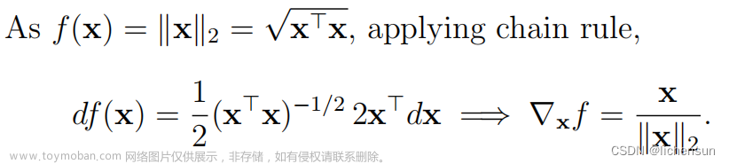
自动微分法计算：

import torch
x = torch.tensor([1.0, 2.0], requires_grad=True)     
y = torch.norm(x)           # y is a fn of x
y                           # tensor(2.2361), torch.sqrt(torch.tensor(5.0))
#使用backward方法对y进行求导，即计算y相对于x的梯度
y.backward()                # take gradient of y w.r.t. x by backward method

x.grad                      # tensor([0.4472, 0.8944])
#检查计算得到的梯度是否与手动计算的梯度相等，结果应为tensor([True, True])
x.grad == x/torch.norm(x)   # tensor([True, True])

x = torch.tensor([0.0, 0.0], requires_grad=True)
y = torch.norm(x)
y.backward()  #对y进行求导。
x.grad
#应为tensor([nan, nan])，因为在零向量上无法计算标准化。
#实际输出：tensor([0., 0.])

x = torch.tensor(0.0, requires_grad=True)
y = torch.abs(x)
y.backward()
x.grad
#输出：tensor(0.)

因此，梯度是x的单位向量。在x = 0处的梯度在数学上是未定义的，但是自动微分返回零。要小心，在这种情况下可能会出现差异。

示例的数量不能除以批处理大小？

import random
import torch
from d2l import torch as d2l

data = d2l.SyntheticRegressionData(w=torch.tensor([2, -3.4]), b=4.2)
data.num_train                         # 1000          
len(data.train_dataloader())           # 32, 1000 / 32 = 31.25
X, y = next(iter(data.train_dataloader()))
X.shape                                # torch.Size([32, 2])
y.shape                                # torch.Size([32, 1])

for i, batch in enumerate(data.train_dataloader()):
    print(i, len(batch[0]))
# first 31 batches contain 32 examples each, last batch contain only 8

# https://pytorch.org/docs/stable/data.html
@d2l.add_to_class(d2l.DataModule)  #@save
def get_tensorloader(self, tensors, train, indices=slice(0, None)):
    tensors = tuple(a[indices] for a in tensors)
    dataset = torch.utils.data.TensorDataset(*tensors)
    return torch.utils.data.DataLoader(dataset, self.batch_size, shuffle=train,
                                       drop_last=True)

# drop_last (bool, optional) – set to True to drop last incomplete batch
# if dataset size is not divisible by batch size. If False and dataset size is  
# not divisible by batch size, then last batch will be smaller. (default: False)


len(data.train_dataloader())       # 31, 1000 // 32 = 31
for i, batch in enumerate(data.train_dataloader()):
    print(i, len(batch[0]))
# only 31 batches containing 32 examples each, last batch with 8 is dropped

默认情况下，最后一个小批处理的尺寸将更小。例如，如果将1000个训练例子划分为32的小批，那么前31批将包含32个，而最后一批只有8个。

解决？：

drop last参数设置为True，以删除最后一个不完整的批处理。

2.

不同loss函数下的线性回归实现

import random
import torch
from torch import nn
from d2l import torch as d2l


#数据
data = d2l.SyntheticRegressionData(w=torch.tensor([2, -3.4]), b=4.2)


# MSE loss (Section 3.5.2 "Defining the Loss Function" of textbook)
@d2l.add_to_class(d2l.LinearRegression)  #@save
#使用了@d2l.add_to_class装饰器来将loss方法添加到LinearRegression类中。
#然后，在loss方法中，使用nn.MSELoss来计算预测值y_hat和真实值y之间的均方误差损失。
def loss(self, y_hat, y):
    fn = nn.MSELoss()
    return fn(y_hat, y)

model = d2l.LinearRegression(lr=0.03)
trainer = d2l.Trainer(max_epochs=5)
trainer.fit(model, data) 
w, b = model.get_w_b() 
print(f'error in estimating w: {data.w - w.reshape(data.w.shape)}')
print(f'error in estimating b: {data.b - b}') 


# Change loss fn to L1Loss ( https://pytorch.org/docs/stable/nn.html#loss-functions )
@d2l.add_to_class(d2l.LinearRegression)  #@save
def loss(self, y_hat, y):
    fn = nn.L1Loss()
    return fn(y_hat, y)

model2 = d2l.LinearRegression(lr=0.03)
trainer = d2l.Trainer(max_epochs=5)
trainer.fit(model2, data) 
w, b = model2.get_w_b() 
print(f'error in estimating w: {data.w - w.reshape(data.w.shape)}')
print(f'error in estimating b: {data.b - b}')

MSE损失（通过取目标和输出之间的差值的平方）对离群值更敏感，而L1损失只考虑差值的绝对大小，并且对离群值更有弹性。

deep learning 代码笔记,深度学习,深度学习,笔记,人工智能

Huber的损失结合了MSE和L1损失函数的最佳特性。当目标和输出之间的差值较小时，它减少到MSE损失，但当差值较大时，它等于L1损失。这样，当远离收敛时，它对L1损失等异常值具有鲁棒性，但在接近收敛时，它更稳定，并像MSE损失一样平滑收敛。它在所有点上也都是可微的。δ参数还允许用户控制损失函数对误差大小的敏感性。

交叉熵

参数化的ReLU

deep learning 代码笔记,深度学习,深度学习,笔记,人工智能

pReLU比ReLU更灵活，因为它有一个额外的参数α，可以与模型中的其他参数一起进行训练。当对于x < 0的ReLU函数消失时，对于x < 0的pReLU是非零的，它解决了负输入的“垂死”ReLU问题。它可能比ReLU更有效地解决消失的梯度。

3.

MLP的等价解

MLP中变量的依赖性

dropout

dropout和重量衰减可以同时应用，以减少过拟合。权值衰减限制了权值的大小，而dropout则通过防止对特定节点的过度依赖而提高了泛化。与只使用权重衰减时相比，当dropout与权重衰减一起使用时，验证损失和精度的曲线更平滑，波动更小。文章来源地址https://www.toymoban.com/news/detail-832894.html